LIve Session 2 CLT
Bivin
9/6/2018
Simulator to Demonstrate CLT
Control Parameters
Path <- "D:/University/SMU/Doing_Data_Science/DDS_repository/Doing-Data-Science/Unit1/yob2016.txt"
df_yob = read.table(Path, stringsAsFactors = FALSE,header = FALSE,sep = ";")
#df = read.table("/Users/bivin/Desktop/OLD COMPUTER ARCHIVES/KadAfrica/MSDS/DDS/MSDS 6306/Unit 5/yob2016.txt",stringsAsFactors = FALSE,header = FALSE,sep = ";")
n1 = 10 # sample size per sample for 1st distribution
n2 = 100 # sample size per sample for 2nd distribution (we will compare these distribuions)
simulations = 1000 #number of samples and thus number of xbars we will generate.
mu = 0; # mean parameter for use with normal distribuions
sigma = 1; # standard deviation parameter for use with normal distribuions
df_yob
Data Holder
xbar_holder1 = numeric(simulations) # This will hold all the sample means for the first distribution.
xbar_holder2 = numeric(simulations) # This will hold all the sample means for the second distribution.
Simulate and Store
Generate 1000 samples each of size 10 and find the mean of each sample. Then store each mean in the xbar_holder vector.
for (i in 1:simulations)
{
  sample1 = rnorm(n1,mean = mu, sd = sigma)
  sample2 = rnorm(n2,mean = mu, sd = sigma)
  xbar1 = mean(sample1)
  xbar2 = mean(sample2)
  xbar_holder1[i] = xbar1
  xbar_holder2[i] = xbar2
}
display the distribution of sample means (plot a histogram of the sample means)
par(mfrow = c(2,1))
hist(xbar_holder1, col = "blue", main = paste("Distribution of the sample mean: n = ", n1), xlab = "Dist 1 Sample Means", xlim = c(-4,4))
hist(xbar_holder2, col = "red", main = paste("Distribution of the sample mean: n = ", n2), xlab = "Dist 2 Sample Means", xlim = c(-4,4))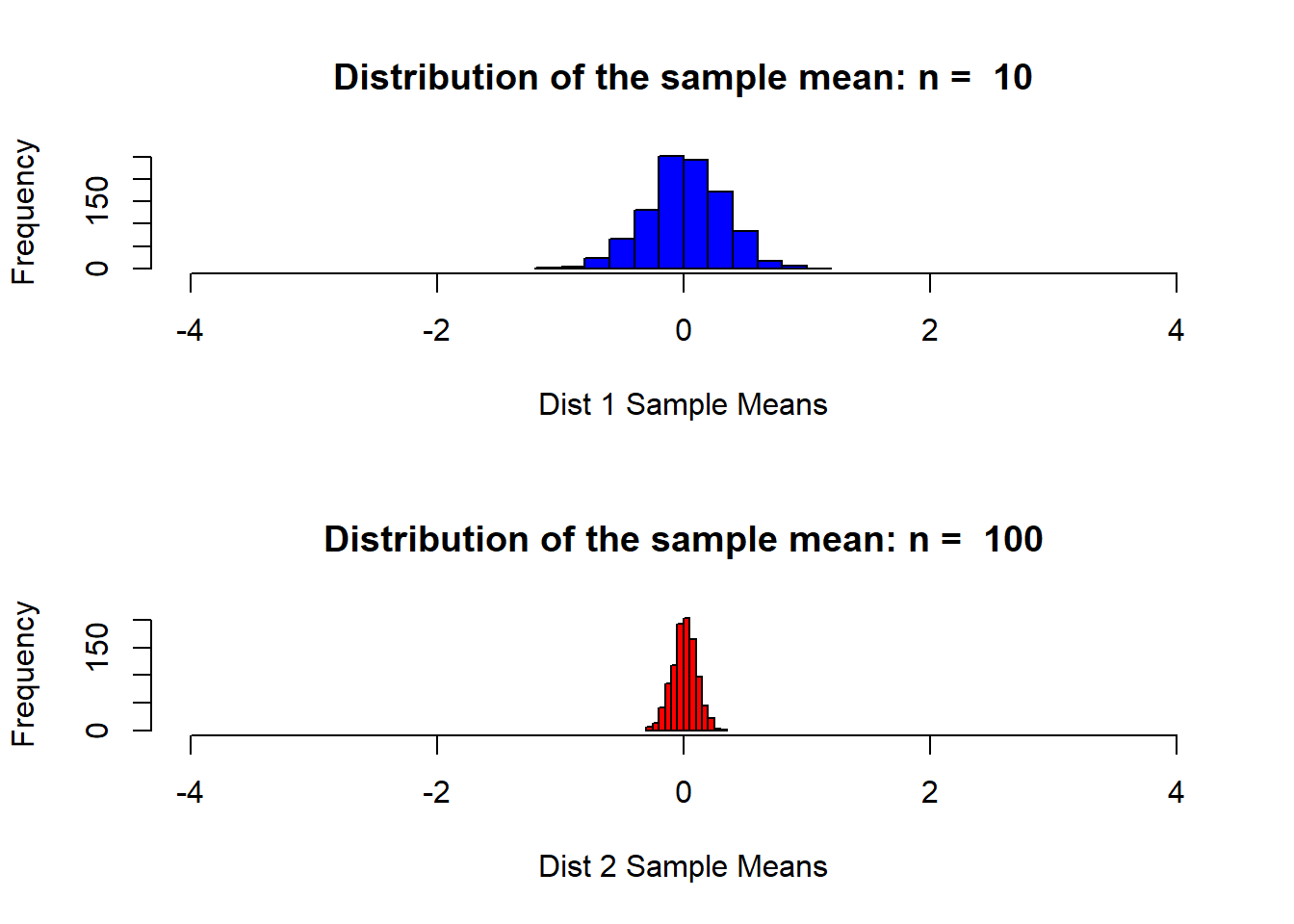
summary statistics of the distribution of the simulated sample means.
summary(xbar_holder1) #5 number summary and the mean## Min. 1st Qu. Median Mean 3rd Qu. Max.
## -1.08993 -0.17721 0.01964 0.01435 0.22762 1.07280summary(xbar_holder2) #5 number summary and the mean## Min. 1st Qu. Median Mean 3rd Qu. Max.
## -0.285790 -0.056127 0.008868 0.008006 0.072489 0.303986sd(xbar_holder1) # standard deviation of dstribuion 1## [1] 0.3137424sd(xbar_holder2) #standard deviation of distribuion 2## [1] 0.09947762