DDS_Final_Project_Code
Adam E.
2023-12-09
ReadMe:
This employee attrition model seeks to analyze the relationship of over 30 variables on employee attrition levels in the Frito Lay Coorporation. Employee attrition is the process whereby a company loses its employees through self election, usually because of a lack of satisfaction or better opportunities elsewhere. Companies spend millions of dollars annually to hire, process, and train talent to make their workforce efficient and productive. Conversely, a talented workforce that is dedicated to a job can increase efficiency in production, reduce workhours, and invite innovation that can save a coorporation millions. Our approach to analyzing the data began with a visual analysis of the impact of certain variables on attrition. The visual analysis was then buttressed with tests using multiple regression models. We then used a stepwise analysis process to identify the most powerful and useful variables to test against attrition. For this study, we used three prediction models, a K to the nearest neighbor (KNN) model, a Naive Bayes model, and a predictive regression model. We tested these models against various variable patterns (using stepwise analysis: Forward, Backward, and Both) to identify which variables had the most statistically significant impact on Attrition rates.
Monthly Income Analysis: The Root Mean Squared Error (RMSE) for this model is 2787.3 (Statistically significant)
Employee Attrition Model:
* Accuracy - the model’s ability to accurately predict Attrition is 83 percent
* Sensitivity – the model’s ability to predict true positives – 70 percent
* Specificity – the model’s ability to predict true negatives – 85.5 percent
Variable Definitions:
Age: Employee age
Attrition: if the employee leaves the job (1 = Yes, 0 = No)
BusinessTravel: The frequency of job travels
DailyRate: Billing cost for employee’s services for a single day
Department: Employee work department
DistanceFromHome: Distance traveled to work from home
Education: Employee education level (1 = Below College, 2 = College, 3 = Bachelor, 4 = Master, 5 = Doctor)
EducationField: Employee education field
EmployeeCount: Employee Count (Constant)
EmployeeNumber: Employee ID
EnvironmentSatisfaction: Num value for environment satisfaction (1 = Low, 2 = Medium, 3 = High, 4 = Very High)
Gender: Employee gender
HourlyRate: The amount of money that employee earns for every hour worked
JobInvolvement: Numerical value for job involvement (1 = Low, 2 = Medium, 3 = High, 4 = Very High)
JobLevel: Numerical value for job level
JobRole: Employee job position
JobSatisfaction: Numerical value for job satisfaction (1 = Low, 2 = Medium, 3 = High, 4 = Very High)
MaritalStatus: Employee marital status
MonthlyIncome: The amount of money that employee earns in one month, before taxes or deductions
MonthlyRate: Billing cost for employee’s services for a month
NumCompaniesWorked: Number of companies worked at
Over18: if employee is over 18 years old
OverTime: if employee works overtime
PercentSalaryHike: Percent increase in salary
PerformanceRating: Numerical value for performance rating (1 = Low, 2 = Good, 3 = Excellent, 4 = Outstanding)
RelationshipSatisfaction: Numerical value for relationship satisfaction (1 = Low, 2 = Medium, 3 = High, 4 = Very High)
StandardHours: Hours employee spent working (Constant)
StockOptionsLevel: Numerical value for stock options
TotalWorkingYears: Total number of years employee worked
TrainingTimesLastYear: Hours employee spent on training last year
WorkLifeBalance: Numerical value for work life balance (1 = Bad, 2 = Good, 3 = Better, 4 = Best)
YearsAtCompany: Number of years employee worked at company
YearsInCurrentRole: Number of years employee worked as their current job role
YearsSinceLastPromotion: Number of years since last promotion
YearsWithCurrentManager: Number of years employee worked with current manager
These models draw on code chuncks from sources such as SMU’s DDS class lectures, Internet Sources, such as (https://bradleyboehmke.github.io/HOML/knn.html, https://rpubs.com/mary18/929056, https://rpubs.com/hanifahpl/emp_att, https://www.datacamp.com/tutorial/k-nearest-neighbors-knn-classification-with-r-tutorial), and chatGPT.
Packages
Data Import from csv
# Read in Data
Path <- "D:/University/SMU/Doing_Data_Science/DDS_repository/DDS_Final_project/CaseStudy2DDS/Attrition_Datasets/CaseStudy2-FallData.csv"
attrition_Data = read.csv(Path, header=TRUE)

# Drop because they are irrelavant and only have one option
attrition_Data <- attrition_Data[, !names(attrition_Data) %in% c("Over18", "EmployeeCount", "StandardHours", "TravelNum")]
attrition_Data
attrition_Data$Attrition = factor(attrition_Data$Attrition, levels = c("Yes", "No"))
# create an alternative model for regression
attrition_Data3 <- attrition_Data
convert_to_numeric <- function(x) {
as.numeric(factor(x, levels = unique(x)))
}
attrition_Data3 <- attrition_Data3 %>%
mutate(Attrition = ifelse(Attrition == 'Yes', 1, 0),
OverTime = ifelse(OverTime == 'Yes', 1, 0),
Gender = ifelse(Gender=='Female', 1, 0)) %>%
mutate_at(vars(BusinessTravel, OverTime, MaritalStatus, Department, EducationField, JobRole), convert_to_numeric)
attrition_Data$WorkLifeBalance2 <- factor(attrition_Data$WorkLifeBalance,
levels = c(1, 2, 3, 4),
labels = c("Bad", "Good", "Better", "Best"))
#---------------------------------read in of no_attrition data ----------------------
# Read in Data
Path2 <- "D:/University/SMU/Doing_Data_Science/DDS_repository/DDS_Final_project/CaseStudy2DDS/Attrition_Datasets/CaseStudy2CompSet_No_Attrition.csv"
attrition_Data_no_attrition = read.csv(Path2, header=TRUE)
# Drop because they are irrelavant and only have one option
attrition_Data_no_attrition <- attrition_Data_no_attrition[, !names(attrition_Data_no_attrition) %in% c("Over18", "Over18Num", "EmployeeCount", "StandardHours", "TravelNum")]
attrition_Data_no_attritionattrition_Data_no_attrition <- attrition_Data_no_attrition %>%
mutate(OverTime = ifelse(OverTime == 'Yes', 1, 0),
Gender = ifelse(Gender=='Female', 1, 0)) %>%
mutate_at(vars(BusinessTravel, OverTime, MaritalStatus, Department, EducationField, JobRole), convert_to_numeric)
attrition_Dataattrition_Data %>%
dplyr::select(Attrition) %>%
group_by(Attrition) %>%
summarise(total_count=n()) %>%
mutate(percentage = (total_count / sum(total_count)) * 100)Visual analysis of the data
# Compute percentages for Attrition
attrition_percentage <- attrition_Data %>%
  dplyr::select(Attrition) %>%
  group_by(Attrition) %>%
  summarise(total_count = n()) %>%
  mutate(percentage = (total_count / sum(total_count)) * 100)

# Create a pie chart with percentage labels
ggplot(attrition_percentage, aes(x = "", y = percentage, fill = Attrition)) +
  geom_bar(stat = "identity", width = 1) +
  coord_polar("y", start = 0) +
  labs(title = "Total Attrition Percentage",
       fill = "Attrition") +
  scale_fill_manual(values = c("Yes" = "red", "No" = "blue")) +
  theme_bw() +
  geom_text(aes(label = paste0(round(percentage), "%")),
            position = position_stack(vjust = 0.5), size = 4, color = "white")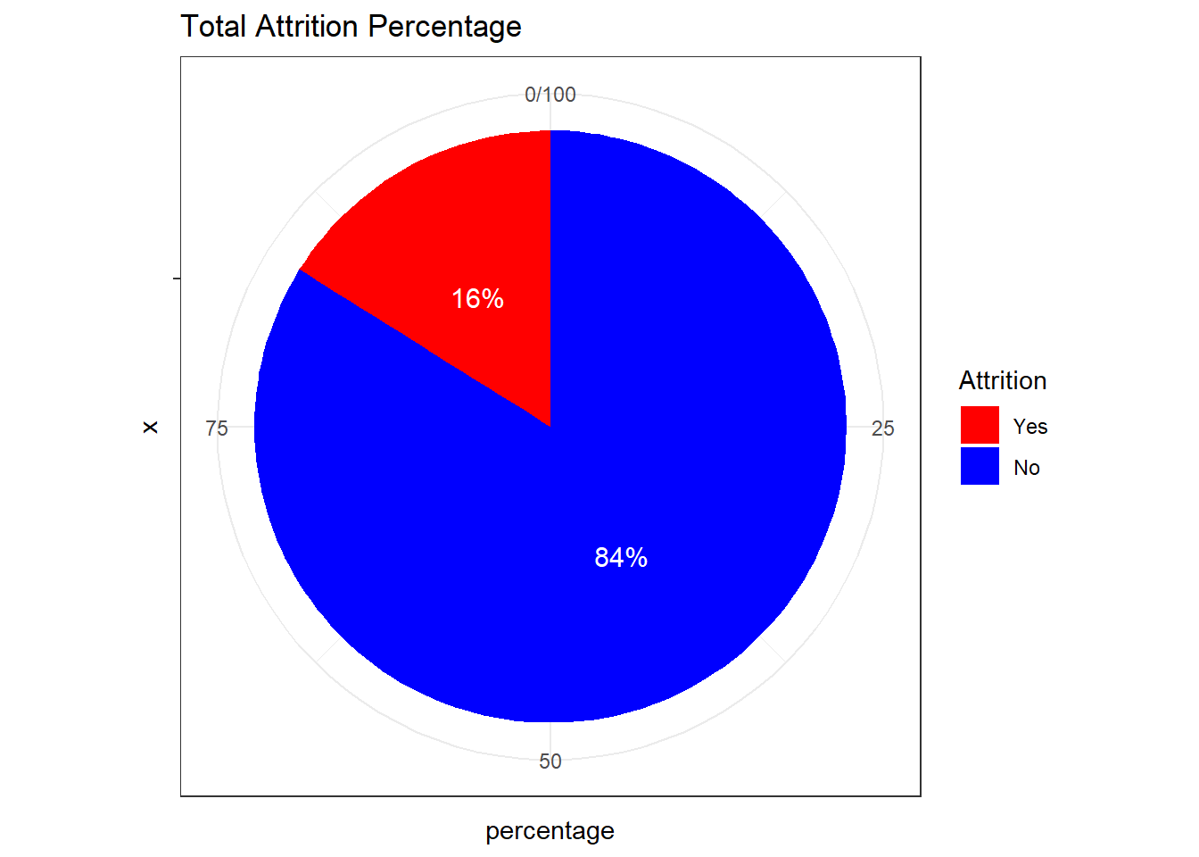
# library(gridExtra)
p1 <- ggplot(attrition_Data) + geom_histogram(aes(Age), binwidth = 5, fill = "blue",col = "black")
p2 <- ggplot(attrition_Data) + geom_histogram(aes(DistanceFromHome), binwidth = 5, fill = "blue",col = "black")
p3 <- ggplot(attrition_Data) + geom_histogram(aes(NumCompaniesWorked), binwidth = 2, fill = "blue",col = "black")
p4 <- ggplot(attrition_Data) + geom_histogram(aes(TotalWorkingYears), binwidth = 4, fill = "blue",col = "black")
p5 <- ggplot(attrition_Data) + geom_histogram(aes(YearsSinceLastPromotion), binwidth = 3, fill = "blue",col = "black")
p6 <- ggplot(attrition_Data) + geom_histogram(aes(TrainingTimesLastYear), binwidth = 1, fill = "blue",col = "black")

grid.arrange(p1, p2, p3, p4, p5, p6, ncol = 3, nrow = 2) 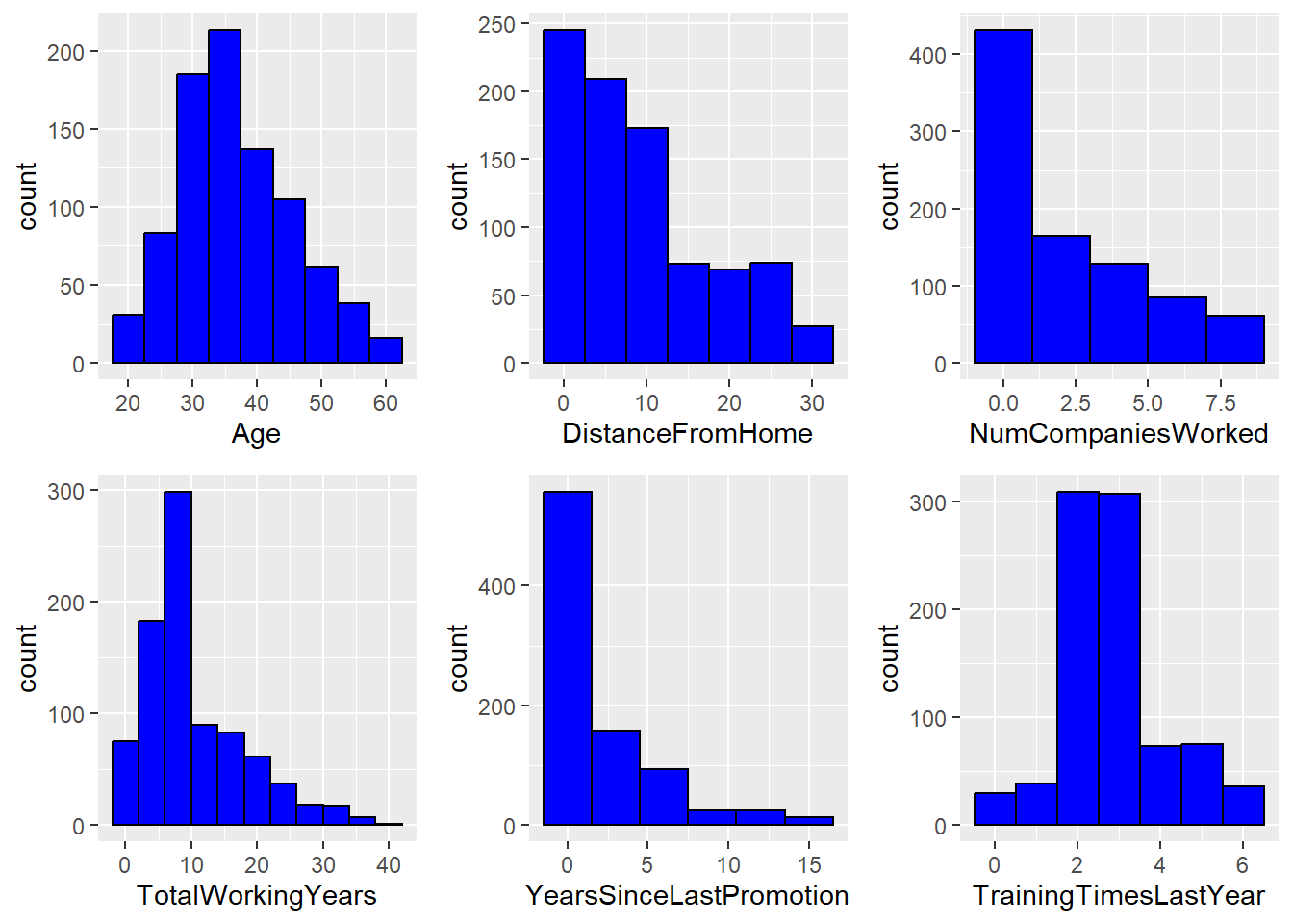
# Filter for specific JobRoles
selected_job_roles <- c("Sales Executive", "Sales Representative", "Manufacturing Director", "Research Scientist", "Manager", "Human Resources", "Labratory Technician")

filtered_data <- attrition_Data %>%
  filter(JobRole %in% selected_job_roles) %>%
    mutate(Age_Group = cut(Age, breaks = c(16, 30, 40, 50, 65),
                         labels = c("16-29", "30-40", "41-50", "50-65"),
                         include.lowest = TRUE))

attrition_Data$WorkLifeBalance2 <- factor(attrition_Data$WorkLifeBalance,
                                                levels = c(1, 2, 3, 4),
                                                labels = c("Bad", "Good", "Better", "Best"))

# Calculate percentages for each JobRole and Overtime
percentage_data <- filtered_data %>%
  group_by(JobRole, OverTime, Attrition) %>%
  summarise(count = n()) %>%
  mutate(percentage = (count / sum(count)) * 100) %>%
  arrange(Attrition)  # Ensure Attrition = Yes is plotted at the bottom
## `summarise()` has grouped output by 'JobRole', 'OverTime'. You can override using the `.groups` argument.# Create bar plot with facets for each JobRole
ggplot(percentage_data, aes(x = OverTime, y = percentage, fill = Attrition)) +
geom_bar(stat = "identity", position = "stack") +
labs(title = "Selected Employee Attrition Status by Overtime and Job Role",
x = "Overtime", y = "Percentage") +
scale_fill_manual(values = c("Yes" = "red", "No" = "blue")) + # Rearranged fill levels
theme_bw() +
facet_wrap(~ JobRole, scales = "free") +
geom_text(aes(label = paste0(round(percentage), "%")),
position = position_stack(vjust = 0.5), size = 3, color = "black")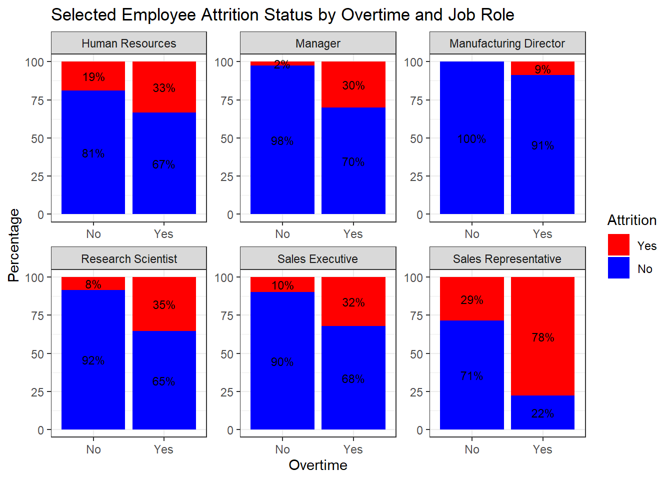
#-----------------------------------------------------------
# Calculate percentages for each JobRole and Age_Group
percentage_data <- filtered_data %>%
  group_by(JobRole, Age_Group, Attrition) %>%
  summarise(count = n()) %>%
  mutate(percentage = (count / sum(count)) * 100) %>%
  arrange(Attrition)  # Ensure Attrition = Yes is plotted at the bottom
## `summarise()` has grouped output by 'JobRole', 'Age_Group'. You can override using the `.groups` argument.# Create bar plot with facets for each JobRole
ggplot(percentage_data, aes(x = Age_Group, y = percentage, fill = Attrition)) +
geom_bar(stat = "identity", position = "stack") +
labs(title = "Selected Employee Attrition Status by Age Group and Job Role",
x = "Age Group", y = "Percentage") +
scale_fill_manual(values = c("Yes" = "red", "No" = "blue")) + # Rearranged fill levels
theme_bw() +
facet_wrap(~ JobRole, scales = "free") +
geom_text(aes(label = paste0(round(percentage), "%")),
position = position_stack(vjust = 0.5), size = 3, color = "black")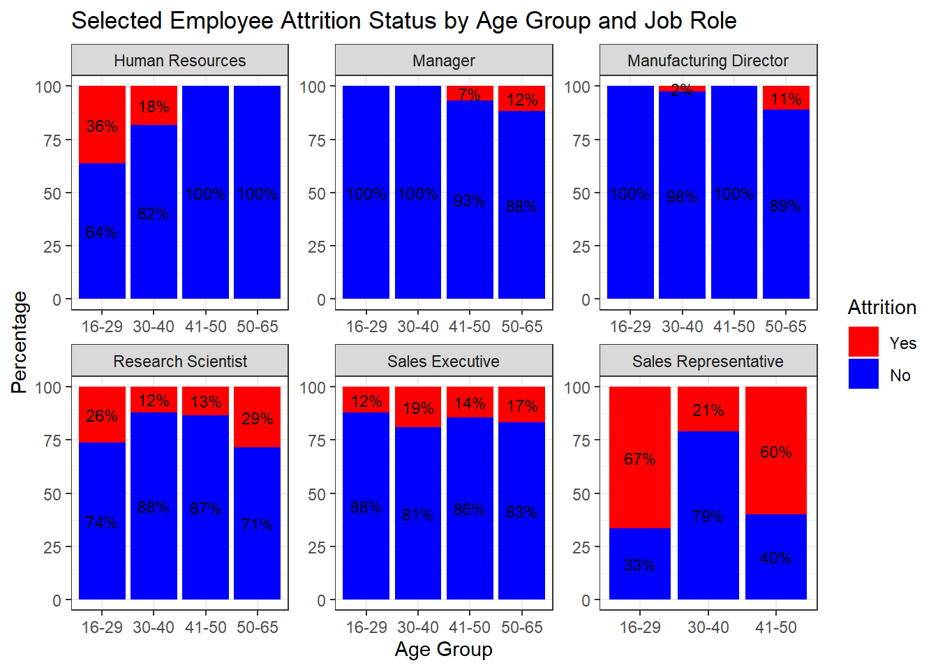
#-------------------------------------------------------------------------
# Calculate percentages for each JobRole and Overtime
percentage_data <- filtered_data %>%
  group_by(JobRole, EnvironmentSatisfaction, Attrition) %>%
  summarise(count = n()) %>%
  mutate(percentage = (count / sum(count)) * 100) %>%
  arrange(Attrition)  # Ensure Attrition = Yes is plotted at the bottom
## `summarise()` has grouped output by 'JobRole', 'EnvironmentSatisfaction'. You can override using the `.groups` argument.# Create bar plot with facets for each JobRole
ggplot(percentage_data, aes(x = EnvironmentSatisfaction, y = percentage, fill = Attrition)) +
geom_bar(stat = "identity", position = "stack") +
labs(title = "Selected Employee Attrition Status by EnvironmentSatisfaction and Job Role",
x = "JobInvolvement", y = "Percentage") +
scale_fill_manual(values = c("Yes" = "red", "No" = "blue")) + # Rearranged fill levels
theme_bw() +
facet_wrap(~ JobRole, scales = "free") +
geom_text(aes(label = paste0(round(percentage), "%")),
position = position_stack(vjust = 0.5), size = 3, color = "black")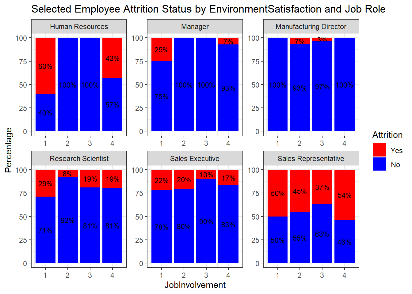
#-----------------------------------------------------------------------------
# Calculate percentages for each JobRole and Overtime
percentage_data <- filtered_data %>%
  group_by(JobRole, JobInvolvement, Attrition) %>%
  summarise(count = n()) %>%
  mutate(percentage = (count / sum(count)) * 100) %>%
  arrange(Attrition)  # Ensure Attrition = Yes is plotted at the bottom
## `summarise()` has grouped output by 'JobRole', 'JobInvolvement'. You can override using the `.groups` argument.# Create bar plot with facets for each JobRole
ggplot(percentage_data, aes(x = JobInvolvement, y = percentage, fill = Attrition)) +
geom_bar(stat = "identity", position = "stack") +
labs(title = "Selected Employee Attrition Status by JobInvolvement and Job Role",
x = "JobInvolvement", y = "Percentage") +
scale_fill_manual(values = c("Yes" = "red", "No" = "blue")) + # Rearranged fill levels
theme_bw() +
facet_wrap(~ JobRole, scales = "free") +
geom_text(aes(label = paste0(round(percentage), "%")),
position = position_stack(vjust = 0.5), size = 3, color = "black")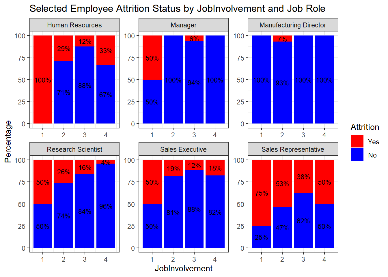
#--------------------------------------------------------------------------------

attrition_Data$WorkLifeBalance2 <- factor(attrition_Data$WorkLifeBalance,
                                                levels = c(1, 2, 3, 4),
                                                labels = c("Bad", "Good", "Better", "Best"))

# Calculate percentages for each JobRole and Overtime
percentage_data <- filtered_data %>%
  group_by(JobRole, WorkLifeBalance2, Attrition) %>%
  summarise(count = n()) %>%
  mutate(percentage = (count / sum(count)) * 100) %>%
  arrange(Attrition)  # Ensure Attrition = Yes is plotted at the bottom
## `summarise()` has grouped output by 'JobRole', 'WorkLifeBalance2'. You can override using the `.groups` argument.# Create bar plot with facets for each JobRole
ggplot(percentage_data, aes(x = WorkLifeBalance2, y = percentage, fill = Attrition)) +
geom_bar(stat = "identity", position = "stack") +
labs(title = "Selected Employee Attrition Status by WorkLifeBalance and Job Role",
x = "WorkLifeBalance", y = "Percentage") +
scale_fill_manual(values = c("Yes" = "red", "No" = "blue")) + # Rearranged fill levels
theme_bw() +
facet_wrap(~ JobRole, scales = "free") +
geom_text(aes(label = paste0(round(percentage), "%")),
position = position_stack(vjust = 0.5), size = 3, color = "black")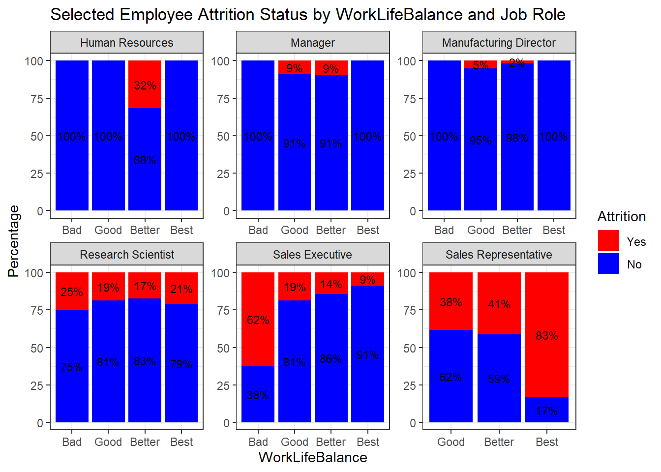
#---------------------------------------------------------------------------------------

attrition_Data$Attrition = factor(attrition_Data$Attrition, levels = c("Yes", "No"))

attrition_Data %>%
  dplyr::group_by(JobRole, Attrition) %>%
  dplyr::summarise(cnt = n()) %>%
  dplyr::mutate(freq = (cnt / sum(cnt))*100) %>%
  ggplot(aes(x = JobRole, y = freq, fill = Attrition)) +
  geom_bar(position = position_stack(), stat = "identity", width = .7) +
  geom_text(aes(label = paste0(round(freq,0), "%")),
            position = position_stack(vjust = 0.5), size = 3) +
  scale_y_continuous(labels = function(x) paste0(x, "%")) +
  labs(title = "Job Role and Attrition", x = "Job Role", y = "Percentage") +
  scale_fill_manual(values = c("red",  "blue")) +
  theme(axis.text.x = element_text(angle = 20, hjust = 0.5))
## `summarise()` has grouped output by 'JobRole'. You can override using the `.groups` argument.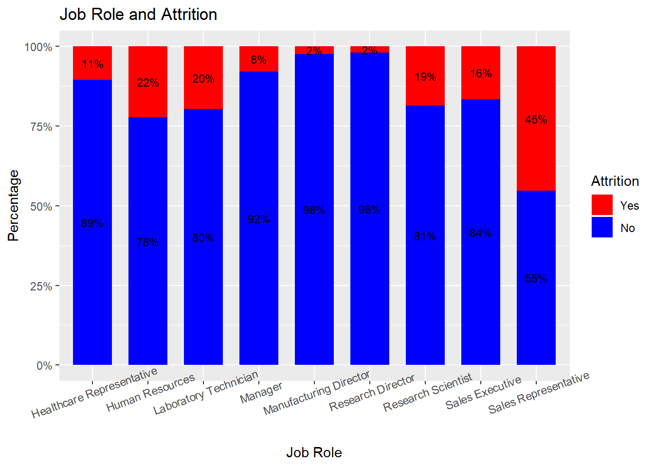
#-------------------------------------------------------------------------------------

attrition_Data %>%
  dplyr::group_by(JobInvolvement, Attrition) %>%
  dplyr::summarise(cnt = n()) %>%
  dplyr::mutate(freq = (cnt / sum(cnt))*100) %>%
  ggplot(aes(x = JobInvolvement, y = freq, fill = Attrition)) +
  geom_bar(position = position_stack(), stat = "identity", width = .7) +
  geom_text(aes(label = paste0(round(freq,0), "%")),
            position = position_stack(vjust = 0.5), size = 3) +
  scale_y_continuous(labels = function(x) paste0(x, "%")) +
  labs(title = "JobInvolvement and Attrition", x = "JobInvolvement", y = "Percentage") +
  scale_fill_manual(values = c("red",  "blue")) +
  theme(axis.text.x = element_text(angle = 20, hjust = 0.5))
## `summarise()` has grouped output by 'JobInvolvement'. You can override using the `.groups` argument.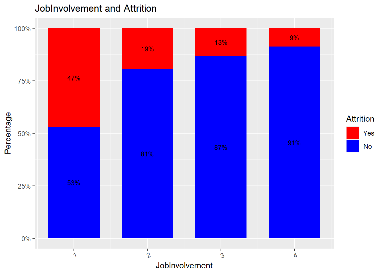
attrition_Data %>%
  dplyr::group_by(Department, Attrition) %>%
  dplyr::summarise(cnt = n()) %>%
  dplyr::mutate(freq = (cnt / sum(cnt))*100) %>%
  ggplot(aes(x = Department, y = freq, fill = Attrition)) +
  geom_bar(position = position_stack(), stat = "identity", width = .7) +
  geom_text(aes(label = paste0(round(freq,0), "%")),
            position = position_stack(vjust = 0.5), size = 3) +
  scale_y_continuous(labels = function(x) paste0(x, "%")) +
  labs(title = "Department and Attrition", x = "Department", y = "Percentage") +
  scale_fill_manual(values = c("red",  "blue")) +
  theme(axis.text.x = element_text(angle = 20, hjust = 0.5))
## `summarise()` has grouped output by 'Department'. You can override using the `.groups` argument.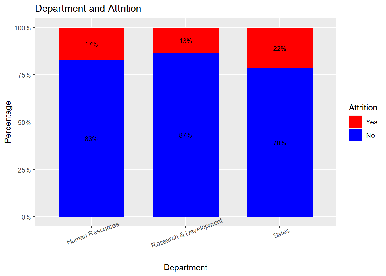
attrition_Data %>%
  dplyr::group_by(NumCompaniesWorked, Attrition) %>%
  dplyr::summarise(cnt = n()) %>%
  dplyr::mutate(freq = (cnt / sum(cnt))*100) %>%
  ggplot(aes(x = NumCompaniesWorked, y = freq, fill = Attrition)) +
  geom_bar(position = position_stack(), stat = "identity", width = .7) +
  geom_text(aes(label = paste0(round(freq,0), "%")),
            position = position_stack(vjust = 0.5), size = 3) +
  scale_y_continuous(labels = function(x) paste0(x, "%")) +
  labs(title = "NumCompaniesWorked and Attrition", x = "NumCompaniesWorked", y = "Percentage") +
  scale_fill_manual(values = c("red",  "blue")) +
  theme(axis.text.x = element_text(angle = 20, hjust = 0.5))
## `summarise()` has grouped output by 'NumCompaniesWorked'. You can override using the `.groups` argument.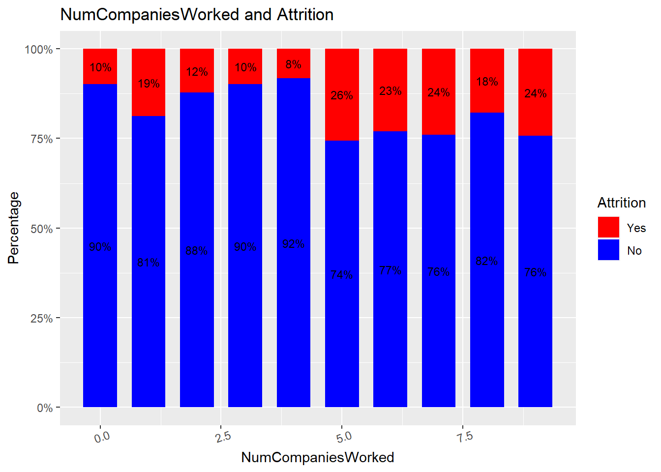
attrition_Data %>%
  dplyr::group_by(OverTime, Attrition) %>%
  dplyr::summarise(cnt = n()) %>%
  dplyr::mutate(freq = (cnt / sum(cnt))*100) %>%
  ggplot(aes(x = OverTime, y = freq, fill = Attrition)) +
  geom_bar(position = position_stack(), stat = "identity", width = .7) +
   geom_text(aes(label = paste0(round(freq,0), "%")),
            position = position_stack(vjust = 0.5), size = 3) +
  scale_y_continuous(labels = function(x) paste0(x, "%")) +
  labs(title = "Over Time and Attrition", x = "Over Time", y = "Percentage") +
  scale_fill_manual(values = c("red",  "blue"))
## `summarise()` has grouped output by 'OverTime'. You can override using the `.groups` argument.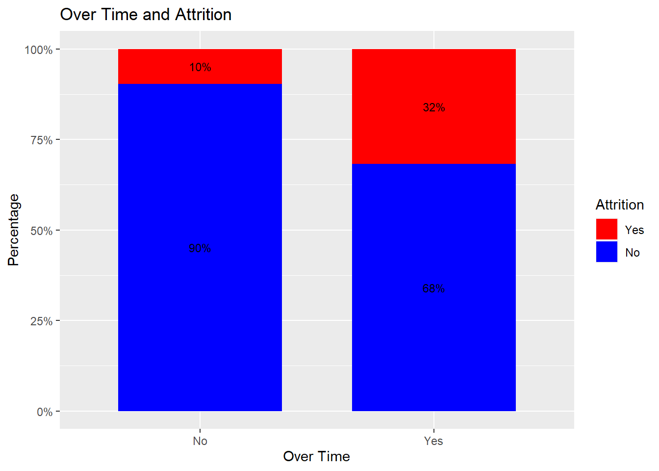
attrition_Data %>%
  dplyr::group_by(MonthlyIncome, Attrition) %>%
  dplyr::summarise(cnt = n()) %>%
  dplyr::mutate(freq = (cnt / sum(cnt)) * 100) %>%
  ggplot(aes(x = Attrition, y = MonthlyIncome, fill = Attrition)) +
  geom_boxplot() +
  labs(title = "Attrition and Monthly Income", x = "Attrition", y = "Monthly Income") +
  scale_fill_manual(values = c("red", "blue"))
## `summarise()` has grouped output by 'MonthlyIncome'. You can override using the `.groups` argument.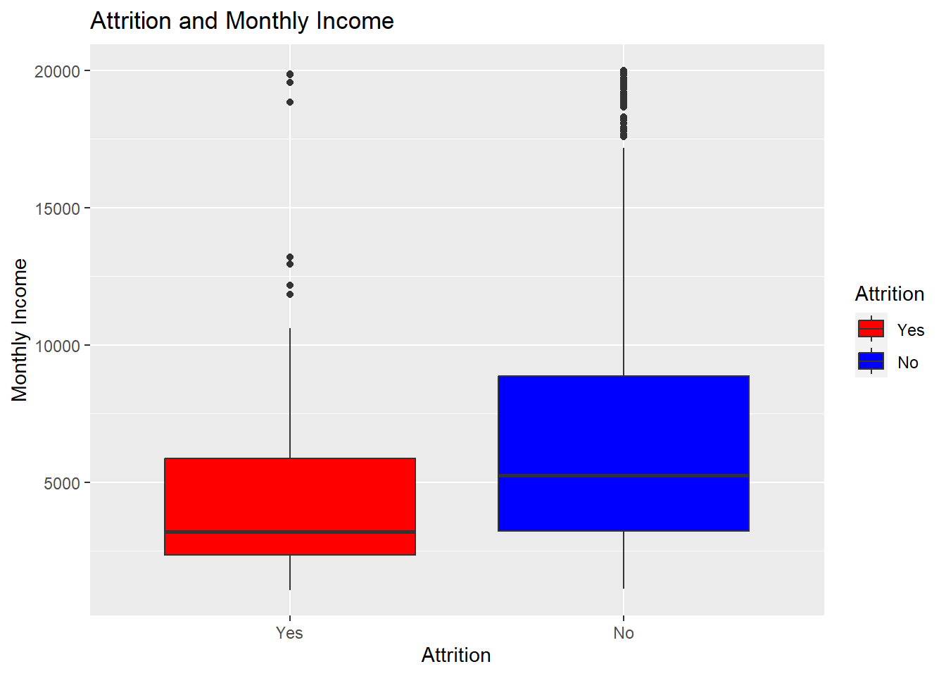
attrition_Data %>%
  dplyr::group_by(HourlyRate, Attrition) %>%
  dplyr::summarise(cnt = n()) %>%
  dplyr::mutate(freq = (cnt / sum(cnt)) * 100) %>%
  ggplot(aes(x = Attrition, y = HourlyRate, fill = Attrition)) +
  geom_boxplot() +
  labs(title = "Attrition and HourlyRate", x = "Attrition", y = "HourlyRate") +
  scale_fill_manual(values = c("red", "blue"))
## `summarise()` has grouped output by 'HourlyRate'. You can override using the `.groups` argument.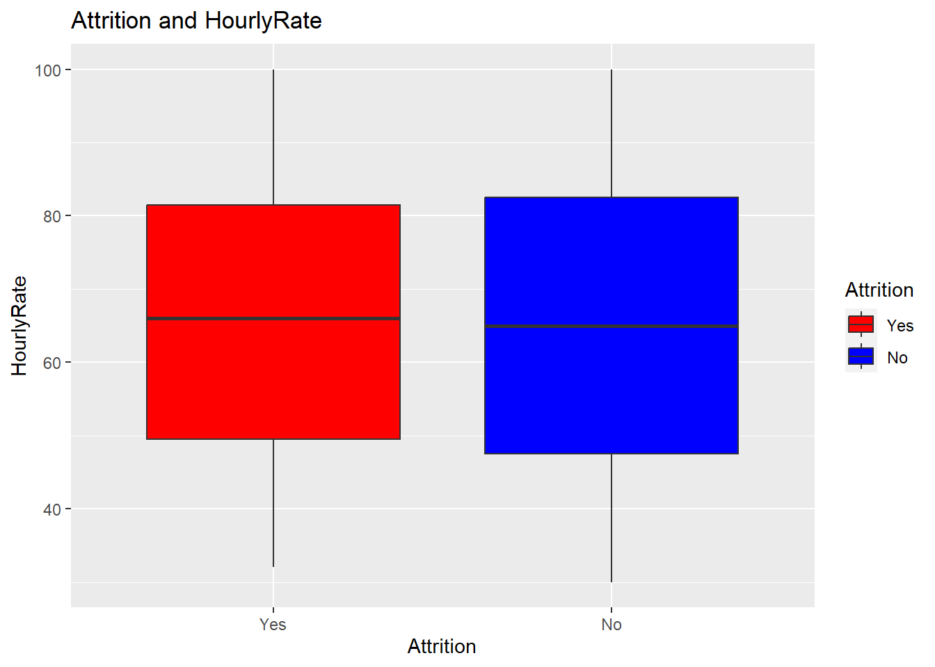
attrition_Data %>%
  dplyr::group_by(MonthlyIncome, JobRole, Attrition) %>%
  dplyr::summarise(cnt = n()) %>%
  dplyr::mutate(freq = (cnt / sum(cnt)) * 100) %>%
  ggplot(aes(x = JobRole, y = MonthlyIncome, fill = Attrition)) +
  geom_boxplot() +
  labs(title = "Monthly Income and Job Role by Attrition", x = "JobRole", y = "Monthly Income") +
  scale_fill_manual(values = c("red", "blue")) +
  theme(axis.text.x = element_text(angle = 45, hjust = 1))  # Rotate x-axis labels
## `summarise()` has grouped output by 'MonthlyIncome', 'JobRole'. You can override using the `.groups` argument.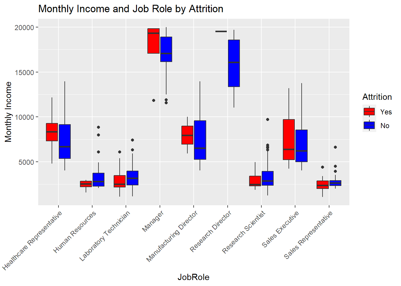
# Create scatterplot with facets for each JobRole
ggplot(filtered_data, aes(x = as.factor(JobSatisfaction), y = MonthlyIncome, color = Attrition, shape = Attrition)) +
  geom_point(position = position_jitter(width = 0.2, height = 0), size = 3) +
  scale_color_manual(values = c("Yes" = "red", "No" = "blue")) +
  scale_shape_manual(values = c("Yes" = 19, "No" = 17)) +
  ylab("Monthly Income") +
  xlab("Job Satisfaction") +
  theme_bw() +
  facet_wrap(~ JobRole, scales = "free") +
  ggtitle("Impact of Income and Satisfaction on Employee Attrition By Position")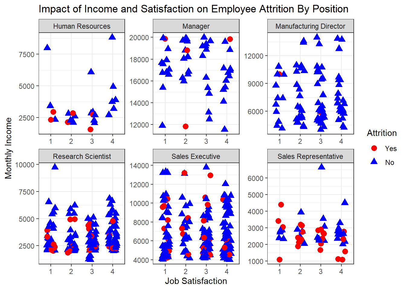
# Create scatterplot with facets for each JobRole for OverTime
ggplot(filtered_data, aes(x = as.factor(YearsSinceLastPromotion), y = MonthlyIncome, color = Attrition, shape = Attrition)) +
  geom_point(position = position_jitter(width = 0.2, height = 0), size = 3) +
  scale_color_manual(values = c("Yes" = "red", "No" = "blue")) +
  scale_shape_manual(values = c("Yes" = 19, "No" = 17)) +
  ylab("Monthly Income") +
  xlab("Years Since Last Promotion") +
  theme_bw() +
  facet_wrap(~ JobRole, scales = "free") +
ggtitle("Impact of Income and Promotion on Employee Attrition By Position") 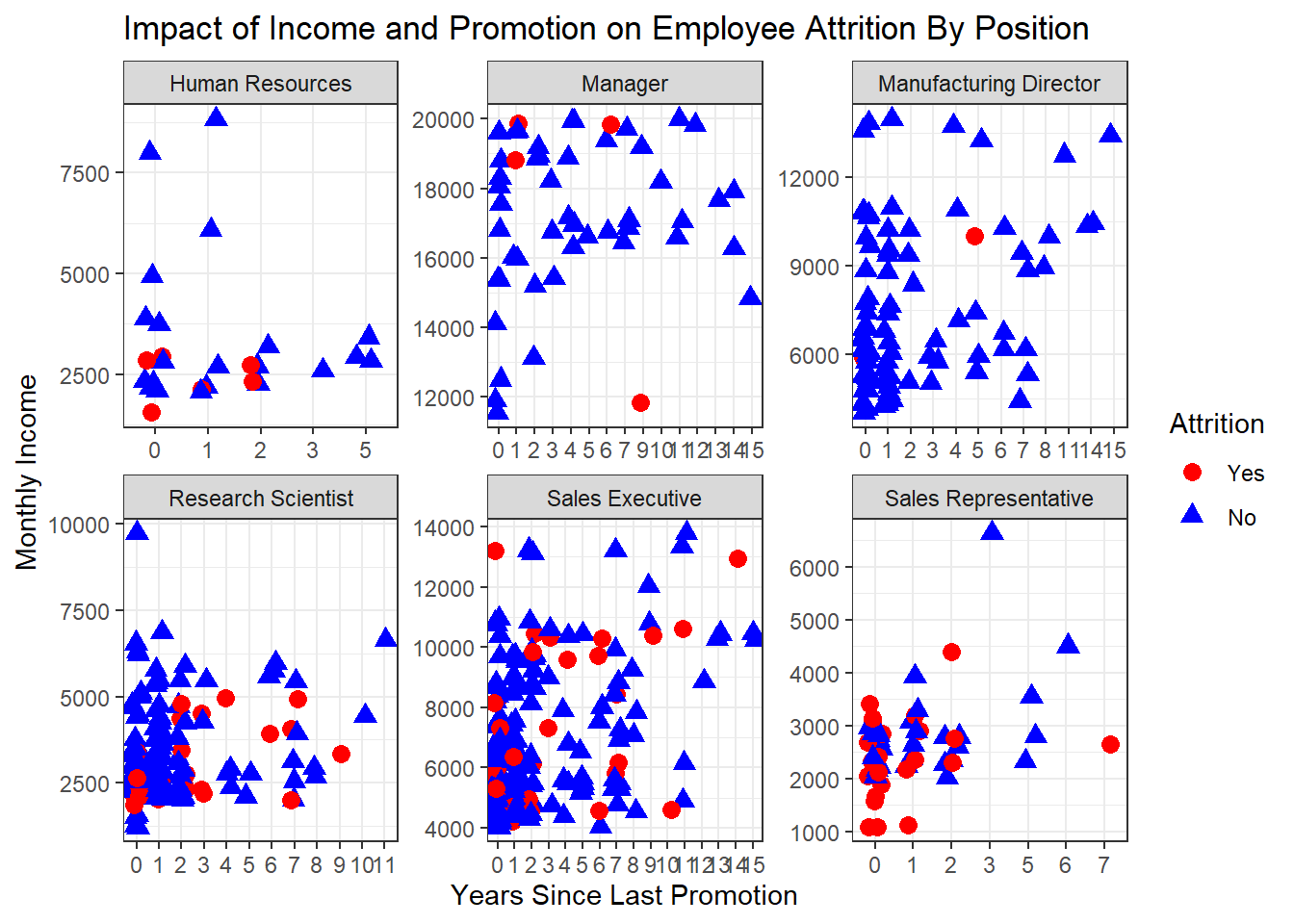
# Bin DistanceFromHome into 5-unit increments
attrition_Data <- attrition_Data %>%
  mutate(DistanceBin = cut(DistanceFromHome, breaks = seq(0, max(DistanceFromHome) + 5, by = 5), right = FALSE))

# Calculate percentages within bins
percentage_DistanceFromHome <- attrition_Data %>%
  group_by(DistanceBin, Attrition) %>%
  summarise(count = n()) %>%
  mutate(percentage = (count / sum(count)) * 100)
## `summarise()` has grouped output by 'DistanceBin'. You can override using the `.groups` argument.# Create the stacked bar plot with labels
ggplot(percentage_DistanceFromHome, aes(x = DistanceBin, y = percentage, fill = Attrition, label = paste(round(percentage, 1), "%"))) +
geom_bar(stat = "identity", position = "stack") +
geom_text(position = position_stack(vjust = 0.5), size = 3, color = "white") +
labs(title = "Employee Attrition Status by Distance From Home",
x = "Distance From Home", y = "Percentage") +
scale_fill_manual(values = c("No" = "blue", "Yes" = "red")) + # Adjust colors if needed
theme_bw()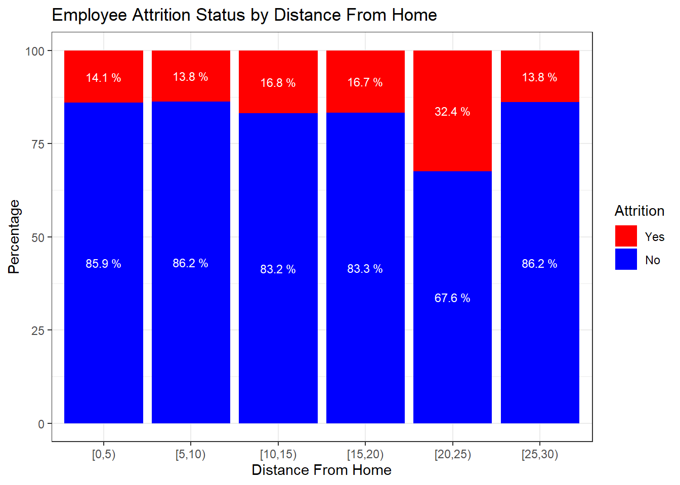
attrition_Data$Attrition = factor(attrition_Data$Attrition, levels = c("Yes", "No"))

attrition_Data %>%
  dplyr::group_by(BusinessTravel, Attrition) %>%
  dplyr::summarise(cnt = n()) %>%
  dplyr::mutate(freq = (cnt / sum(cnt))*100) %>%
  ggplot(aes(x = BusinessTravel, y = freq, fill = Attrition)) +
  geom_bar(position = position_stack(), stat = "identity", width = .7) +
   geom_text(aes(label = paste0(round(freq,0), "%")),
            position = position_stack(vjust = 0.5), size = 3) +
  scale_y_continuous(labels = function(x) paste0(x, "%")) +
  labs(title = "Business Travel and Attrition", x = "Business Travel", y = "Percentage") +
  scale_x_discrete(breaks = c("Travel_Rarely", "Travel_Frequently", "Non-Travel"),
                              labels = c("Travel Rarely","Travel Frequently", "Non Travel")) +
  scale_fill_manual(values = c("red",  "blue")) +
   theme_bw()
## `summarise()` has grouped output by 'BusinessTravel'. You can override using the `.groups` argument.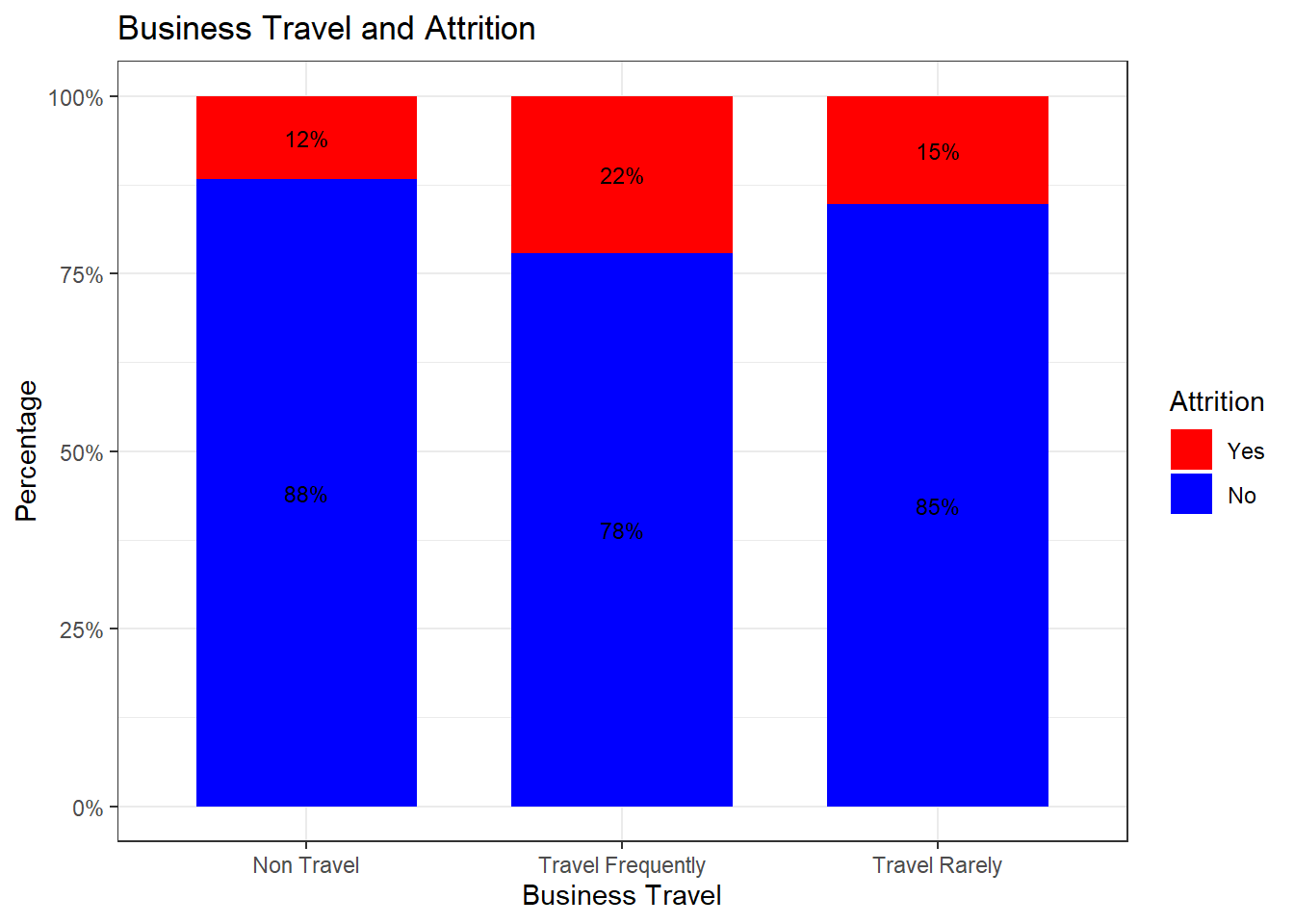
attrition_Data$EnvironmentSatisfaction2 <- factor(attrition_Data$EnvironmentSatisfaction,
                                                levels = c(1, 2, 3, 4),
                                                labels = c("Low", "Medium", "High", "Very High"))

attrition_Data %>%
  dplyr::group_by(EnvironmentSatisfaction2, Attrition) %>%
  dplyr::summarise(cnt = n()) %>%
  dplyr::mutate(freq = (cnt / sum(cnt))*100) %>%
  ggplot(aes(x = EnvironmentSatisfaction2, y = freq, fill = Attrition)) +
  geom_bar(position = position_stack(), stat = "identity", width = .7) +
  geom_text(aes(label = paste0(round(freq,0), "%")),
            position = position_stack(vjust = 0.5), size = 3) +
  scale_y_continuous(labels = function(x) paste0(x, "%")) +
  labs(title = "Environment Satisfaction and Attrition", x = "Environment Satisfaction", y = "Percentage") +
  scale_fill_manual(values = c("red",  "blue")) +
  theme_bw()
## `summarise()` has grouped output by 'EnvironmentSatisfaction2'. You can override using the `.groups` argument.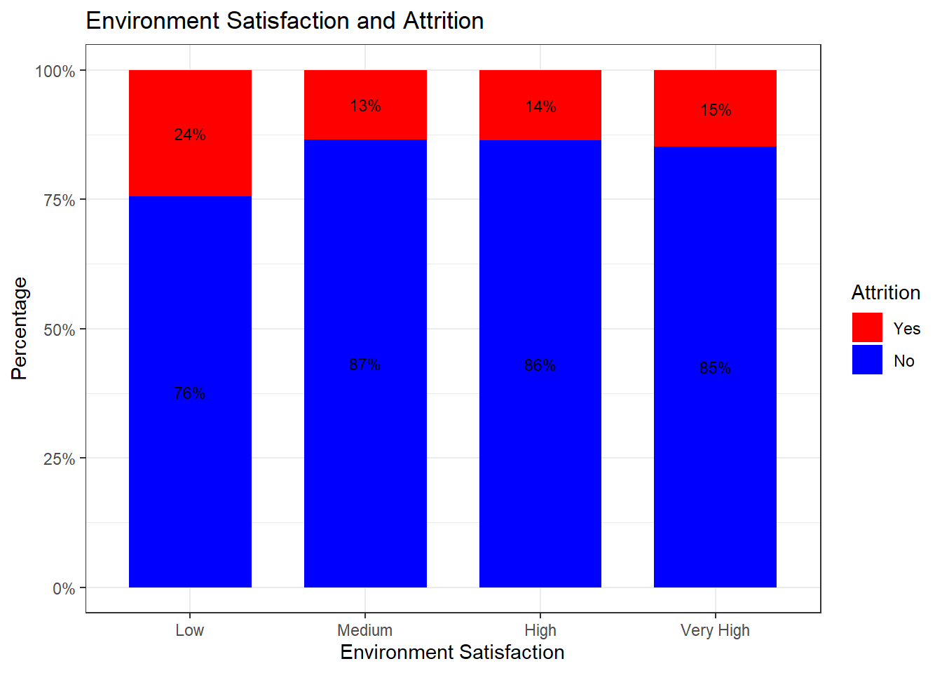
attrition_Data %>%
  dplyr::group_by(JobSatisfaction, Attrition) %>%
  dplyr::summarise(cnt = n()) %>%
  dplyr::mutate(freq = (cnt / sum(cnt))*100) %>%
  ggplot(aes(x = JobSatisfaction, y = freq, fill = Attrition)) +
  geom_bar(position = position_stack(), stat = "identity", width = .7) +
  geom_text(aes(label = paste0(round(freq,0), "%")),
            position = position_stack(vjust = 0.5), size = 3) +
  scale_y_continuous(labels = function(x) paste0(x, "%")) +
  labs(title = "JobSatisfaction and Attrition", x = "JobSatisfaction", y = "Percentage") +
  scale_fill_manual(values = c("red",  "blue")) +
  theme_bw()
## `summarise()` has grouped output by 'JobSatisfaction'. You can override using the `.groups` argument.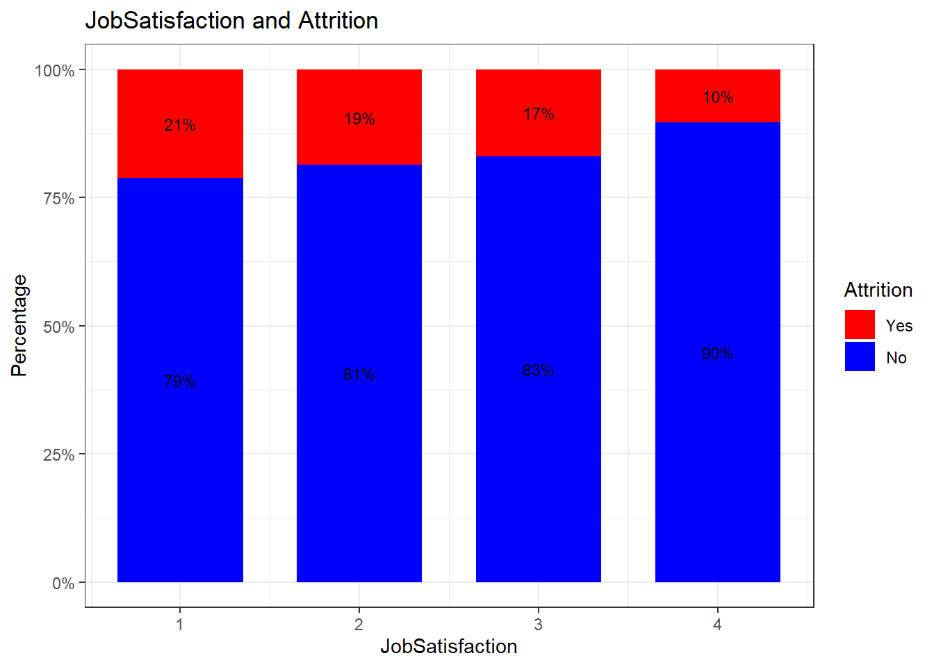
attrition_Data$WorkLifeBalance2 <- factor(attrition_Data$WorkLifeBalance,
                                                levels = c(1, 2, 3, 4),
                                                labels = c("Bad", "Good", "Better", "Best"))
attrition_Data %>%
  dplyr::group_by(WorkLifeBalance2, Attrition) %>%
  dplyr::summarise(cnt = n()) %>%
  dplyr::mutate(freq = (cnt / sum(cnt))*100) %>%
  ggplot(aes(x = WorkLifeBalance2, y = freq, fill = Attrition)) +
  geom_bar(position = position_stack(), stat = "identity", width = .7) +
  geom_text(aes(label = paste0(round(freq,0), "%")),
            position = position_stack(vjust = 0.5), size = 3) +
  scale_y_continuous(labels = function(x) paste0(x, "%")) +
  labs(title = "Work Life Balance and Attrition", x = "Work Life Balance", y = "Percentage") +
  scale_fill_manual(values = c("red",  "blue")) +
  theme_bw()
## `summarise()` has grouped output by 'WorkLifeBalance2'. You can override using the `.groups` argument.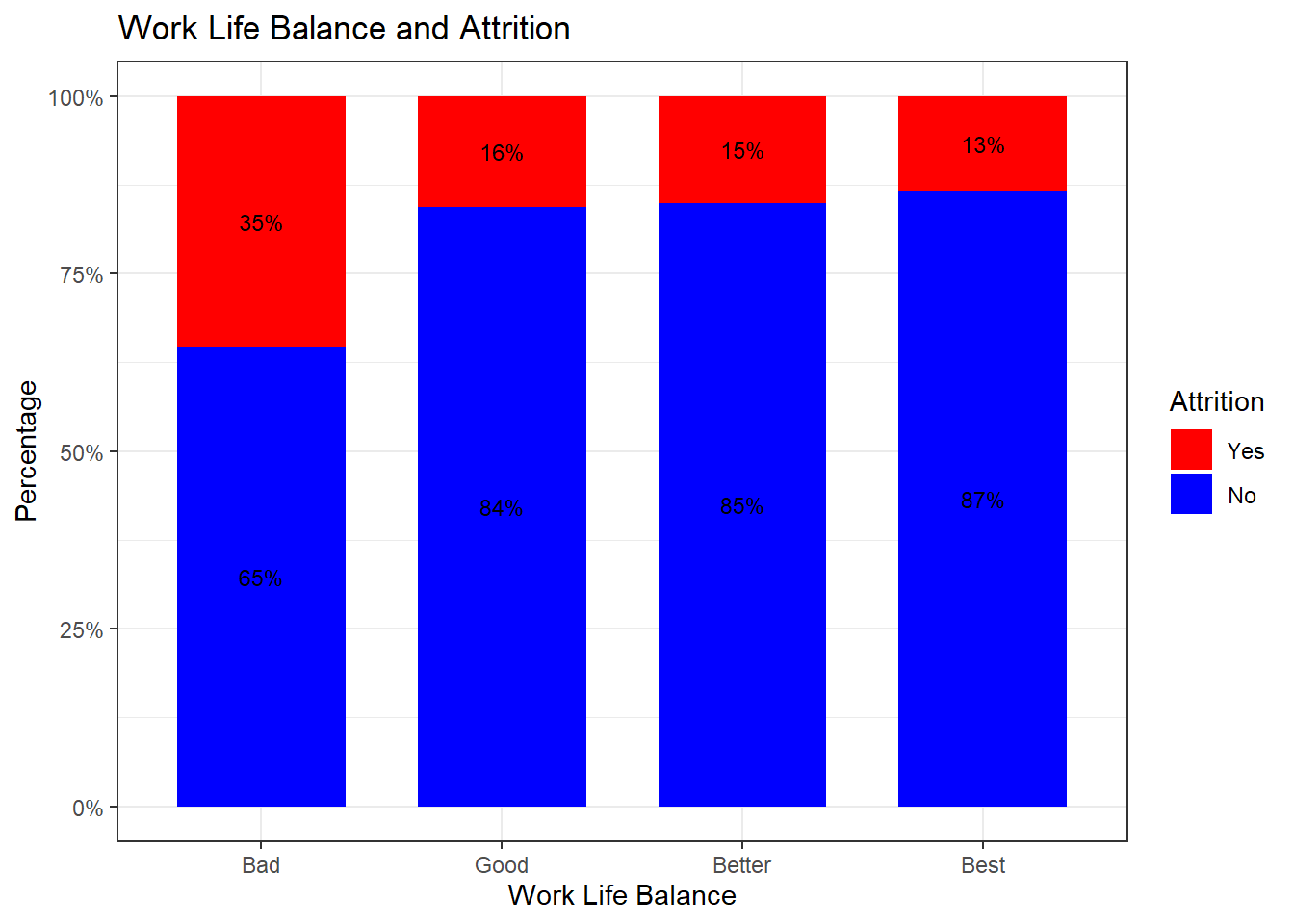
attrition_Data %>%
  dplyr::group_by(YearsSinceLastPromotion, Attrition) %>%
  dplyr::summarise(cnt = n()) %>%
  dplyr::mutate(freq = (cnt / sum(cnt))*100) %>%
  ggplot(aes(x = YearsSinceLastPromotion, y = freq, fill = Attrition)) +
  geom_bar(position = position_stack(), stat = "identity", width = .7) +
  geom_text(aes(label = paste0(round(freq,0), "%")),
            position = position_stack(vjust = 0.5), size = 3) +
  scale_y_continuous(labels = function(x) paste0(x, "%")) +
  labs(title = "YearsSinceLastPromotion and Attrition", x = "YearsSinceLastPromotion", y = "Percentage") +
  scale_fill_manual(values = c("red",  "blue")) +
  theme_bw()
## `summarise()` has grouped output by 'YearsSinceLastPromotion'. You can override using the `.groups` argument.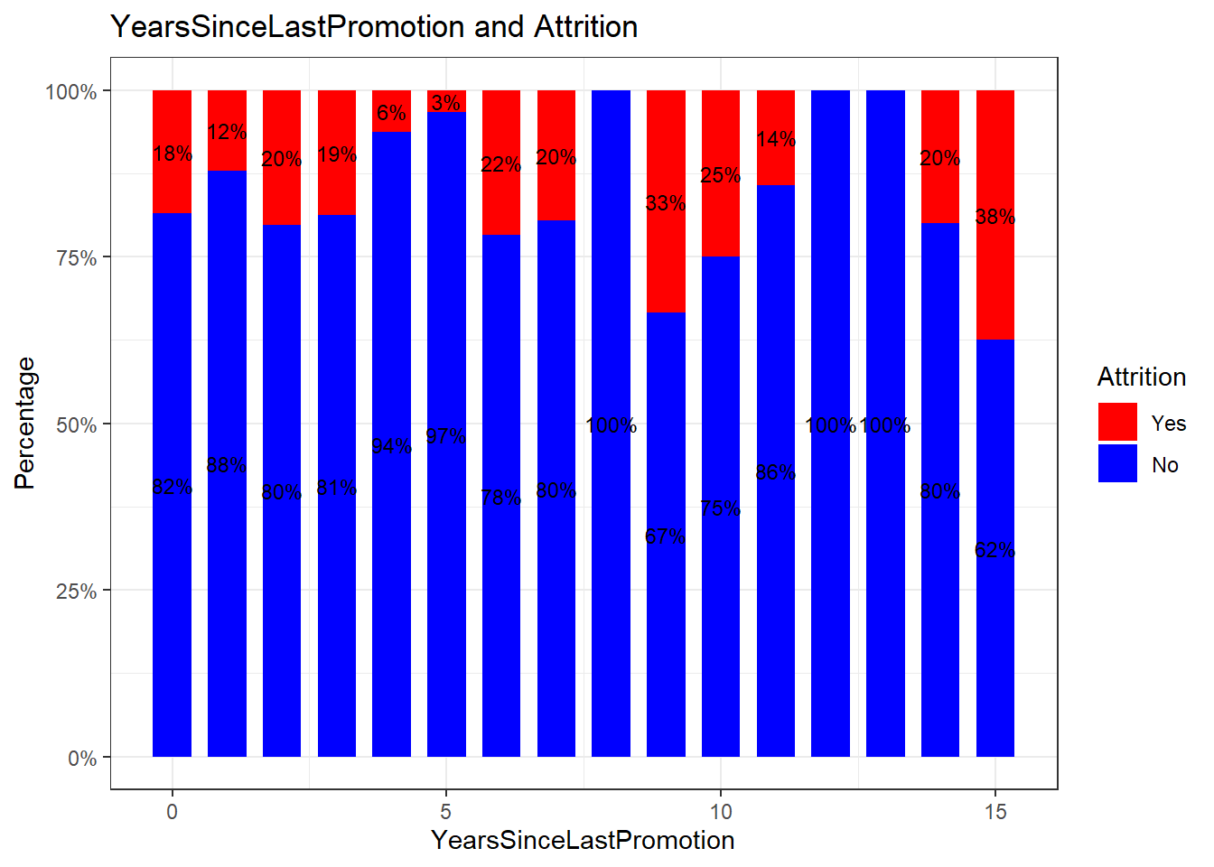
attrition_Data %>%
  dplyr::group_by(TotalWorkingYears, Attrition) %>%
  dplyr::summarise(cnt = n()) %>%
  dplyr::mutate(freq = (cnt / sum(cnt))*100) %>%
  ggplot(aes(x = TotalWorkingYears, y = freq, fill = Attrition)) +
  geom_bar(position = position_stack(), stat = "identity", width = .7) +
  geom_text(aes(label = paste0(round(freq,0), "%")),
            position = position_stack(vjust = 0.5), size = 3) +
  scale_y_continuous(labels = function(x) paste0(x, "%")) +
  labs(title = "TotalWorkingYears and Attrition", x = "TotalWorkingYears", y = "Percentage") +
  scale_fill_manual(values = c("red",  "blue")) +
  theme_bw()
## `summarise()` has grouped output by 'TotalWorkingYears'. You can override using the `.groups` argument.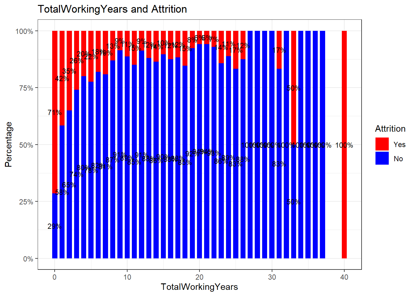
filtered_data <- filtered_data %>%
  mutate(Year_Group = cut(TotalWorkingYears, breaks = c(0, 5, 10, 15, 20, 40),
                          labels = c("0-5", "6-10", "11-15", "16-20", "21-40"),
                          include.lowest = TRUE))

# Calculate percentages for each JobRole and Year_Group
percentage_data <- filtered_data %>%
  group_by(Year_Group, Attrition) %>%
  summarise(count = n()) %>%
  mutate(percentage = (count / sum(count)) * 100) %>%
  arrange(Attrition)  # Ensure Attrition = Yes is plotted at the bottom
## `summarise()` has grouped output by 'Year_Group'. You can override using the `.groups` argument.# Create bar plot with facets for each JobRole
ggplot(percentage_data, aes(x = Year_Group, y = percentage, fill = Attrition)) +
geom_bar(stat = "identity", position = "stack") +
labs(title = "Selected Employee Attrition Status by Years worked",
x = "Years Worked", y = "Percentage") +
scale_fill_manual(values = c("Yes" = "red", "No" = "blue")) + # Rearranged fill levels
theme_bw() +
#facet_wrap(~ JobRole, scales = "free") +
geom_text(aes(label = paste0(round(percentage), "%")),
position = position_stack(vjust = 0.5), size = 3, color = "black")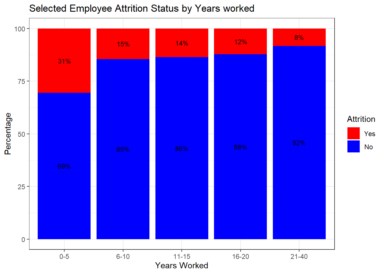
attrition_Data %>%
  dplyr::group_by(Gender, Attrition) %>%
  dplyr::summarise(cnt = n()) %>%
  dplyr::mutate(freq = (cnt / sum(cnt))*100) %>%
  ggplot(aes(x = Gender, y = freq, fill = Attrition)) +
  geom_bar(position = position_stack(), stat = "identity", width = .7) +
   geom_text(aes(label = paste0(round(freq,0), "%")),
            position = position_stack(vjust = 0.5), size = 3) +
  scale_y_continuous(labels = function(x) paste0(x, "%")) +
  labs(title = "Gender and Attrition", x = "Gender", y = "Percentage") +
  scale_fill_manual(values = c("red",  "blue")) +
  theme_bw()
## `summarise()` has grouped output by 'Gender'. You can override using the `.groups` argument.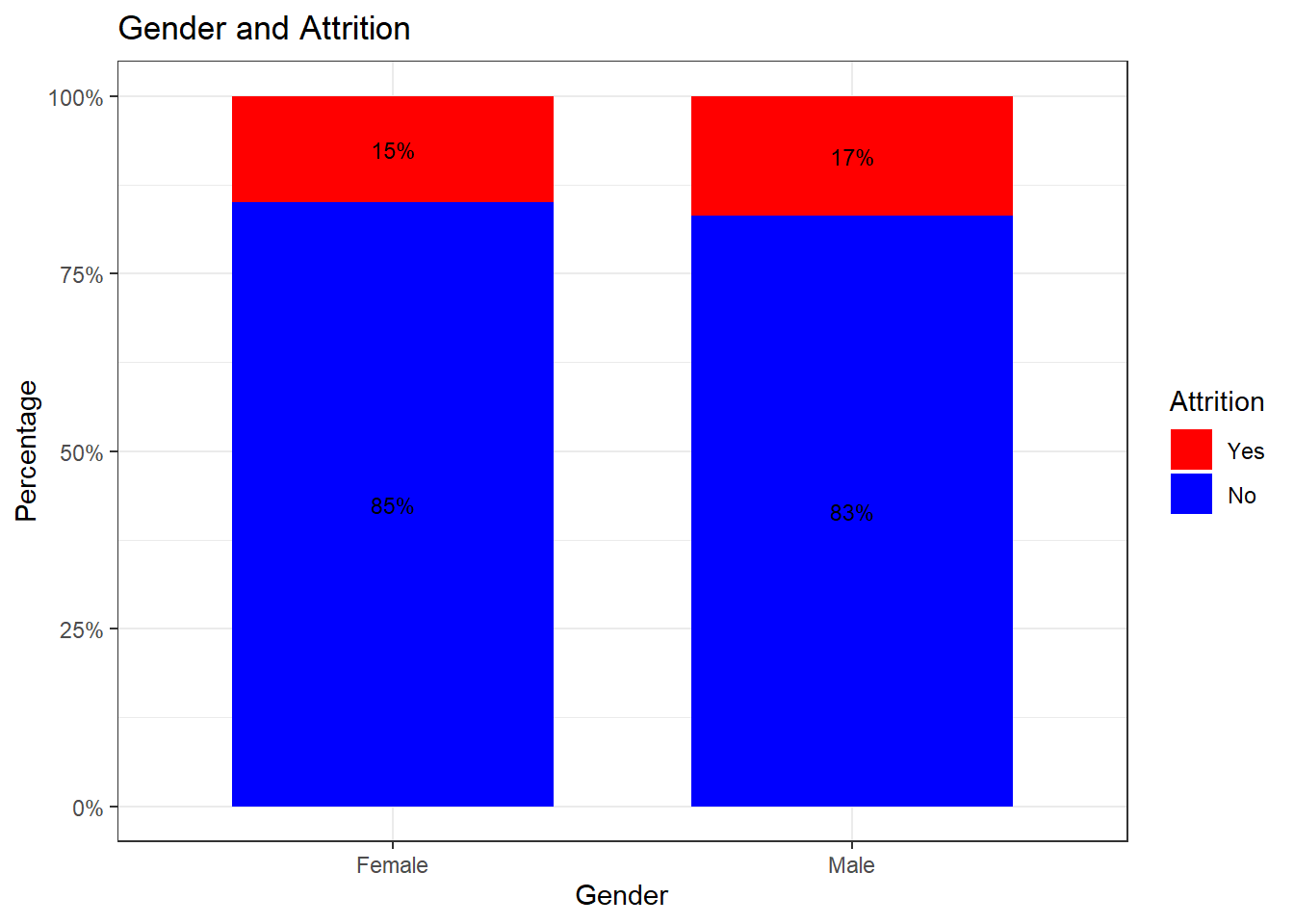
plot_sat_overtime <- ggplot(attrition_Data, aes(x = as.factor(OverTime), y = MonthlyIncome, fill = Attrition))+
                       geom_boxplot()+
                       scale_fill_manual(values = c("Yes" = "red", "No" = "blue")) + # Adjust colors accordingly
                       ylab("Monthly Income")+
                       xlab("Overtime")+
                       theme_bw()+
                       ggtitle("Impact of Monthly income and Overtime On Employee Attrition")
plot_sat_overtime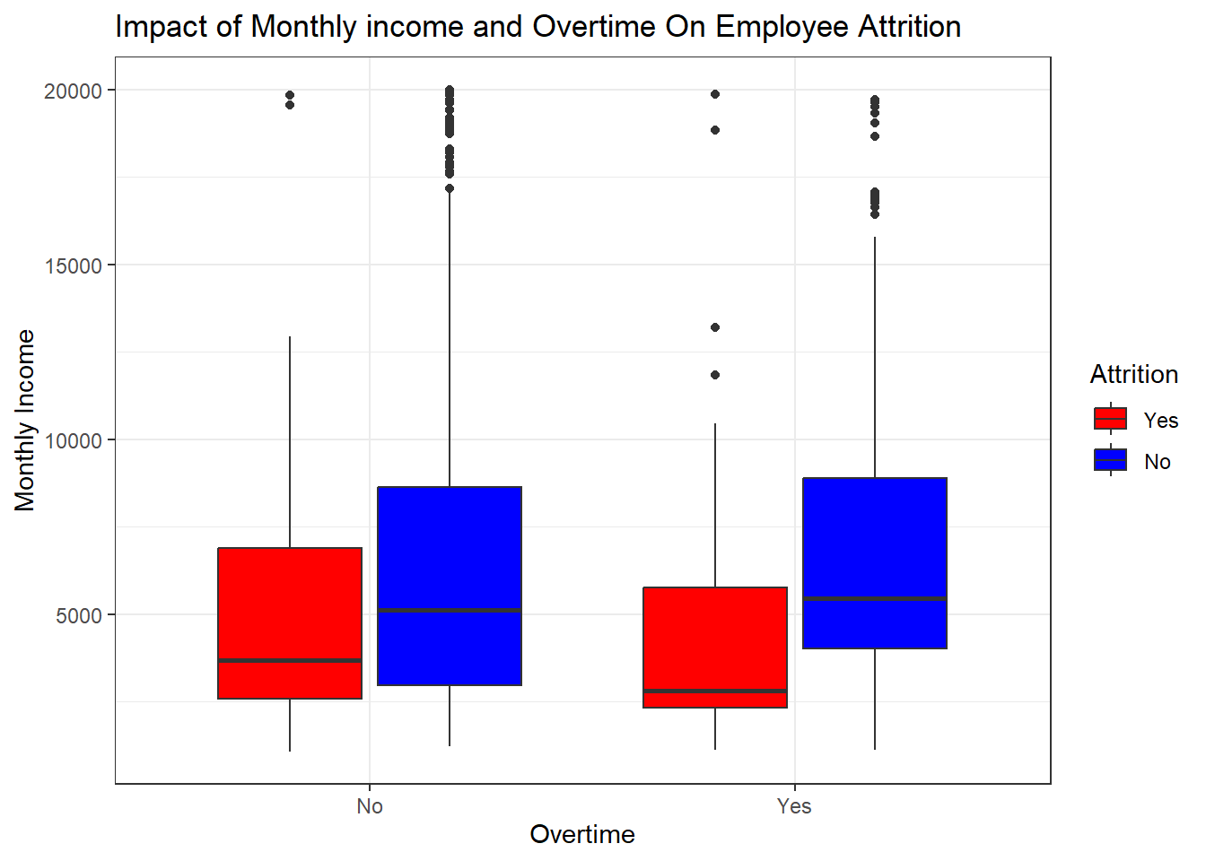
plot_sat_income <- ggplot(attrition_Data, aes(x = as.factor(JobSatisfaction), y = MonthlyIncome, fill = Attrition))+
                       geom_boxplot()+
                       scale_fill_manual(values = c("Yes" = "red", "No" = "blue")) + # Adjust colors accordingly
                       ylab("Monthly Income")+
                       xlab("Job Satisfaction")+
                       theme_bw()+
                       ggtitle("Impact of Monthly income and Job Satisfaction On Employee Attrition")
plot_sat_income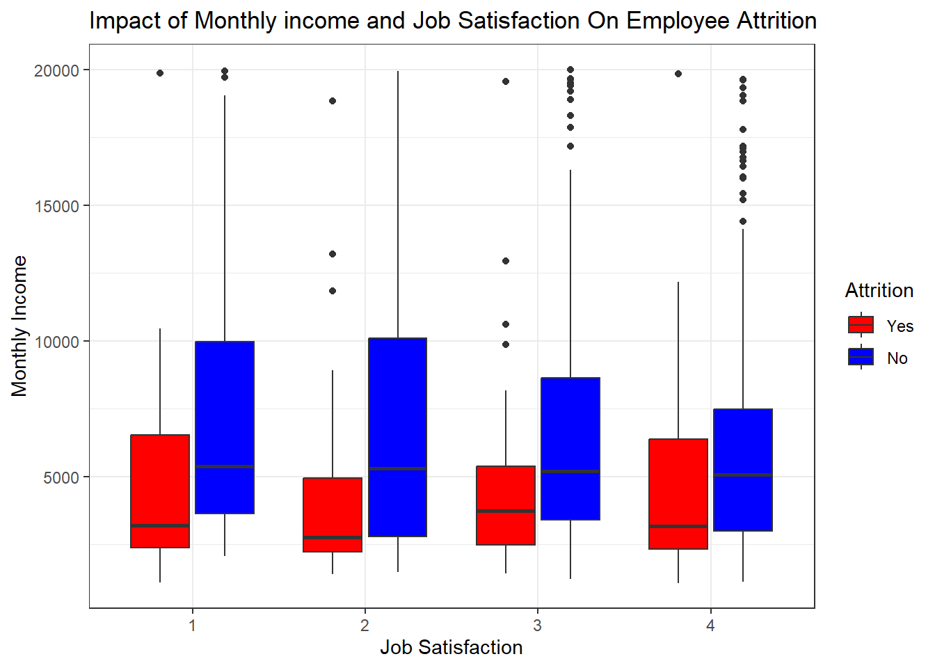
# Create a jittered scatterplot comparing DistanceFromHome by OverTime and Attrition
ggplot(attrition_Data, aes(x = OverTime, y = DistanceFromHome, color = Attrition)) +
  geom_jitter(position = position_jitter(width = 0.3), size = 3) +
  labs(title = "Comparison of Distance From Home by Overtime and Attrition",
       x = "Overtime", y = "Distance From Home") +
  scale_color_manual(values = c("Yes" = "red", "No" = "blue")) +
  theme_bw()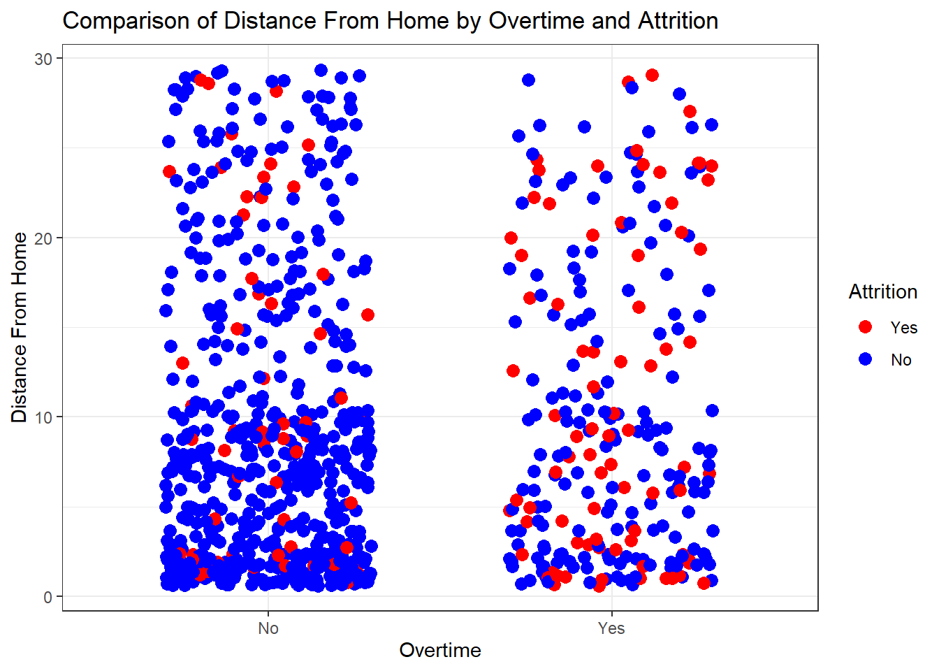
# Grouping by OverTime, MaritalStatus, and Attrition to count occurrences
grouped_data <- attrition_Data %>%
  group_by(OverTime, MaritalStatus, Attrition) %>%
  summarise(count = n(), .groups = "drop")

# Creating a bar plot comparing Marital Status, Overtime, and Attrition
ggplot(grouped_data, aes(x = MaritalStatus, y = count, fill = Attrition)) +
  geom_bar(stat = "identity", position = "dodge") +
  facet_grid(. ~ OverTime) +  # Facet by OverTime
  labs(title = "Comparison of Marital Status, Overtime, and Attrition",
       x = "Marital Status", y = "Count") +
  scale_fill_manual(values = c("Yes" = "red", "No" = "blue")) +
  theme_bw()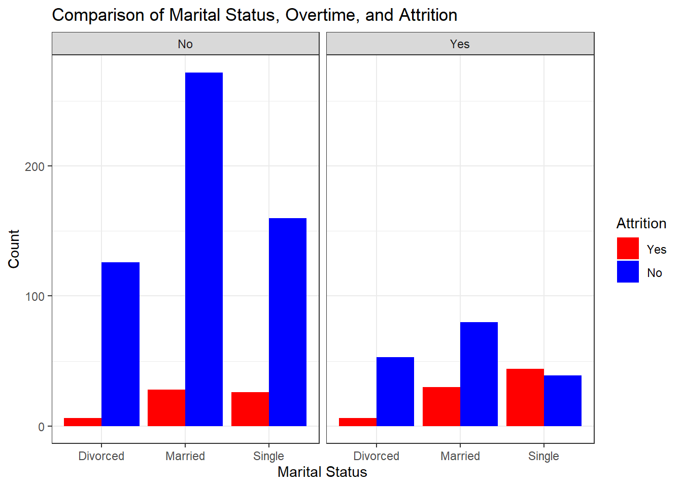
attrition_Data %>%
  dplyr::group_by(MaritalStatus, Attrition) %>%
  dplyr::summarise(cnt = n()) %>%
  dplyr::mutate(freq = (cnt / sum(cnt))*100) %>%
  ggplot(aes(x = MaritalStatus, y = freq, fill = Attrition)) +
  geom_bar(position = position_stack(), stat = "identity", width = .7) +
   geom_text(aes(label = paste0(round(freq,0), "%")),
            position = position_stack(vjust = 0.5), size = 3) +
  scale_y_continuous(labels = function(x) paste0(x, "%")) +
  labs(title = "Comparison of Marital Status and Attrition", x = "Marital Status", y = "Percentage") +
  scale_fill_manual(values = c("red",  "blue")) +
  theme_bw()
## `summarise()` has grouped output by 'MaritalStatus'. You can override using the `.groups` argument.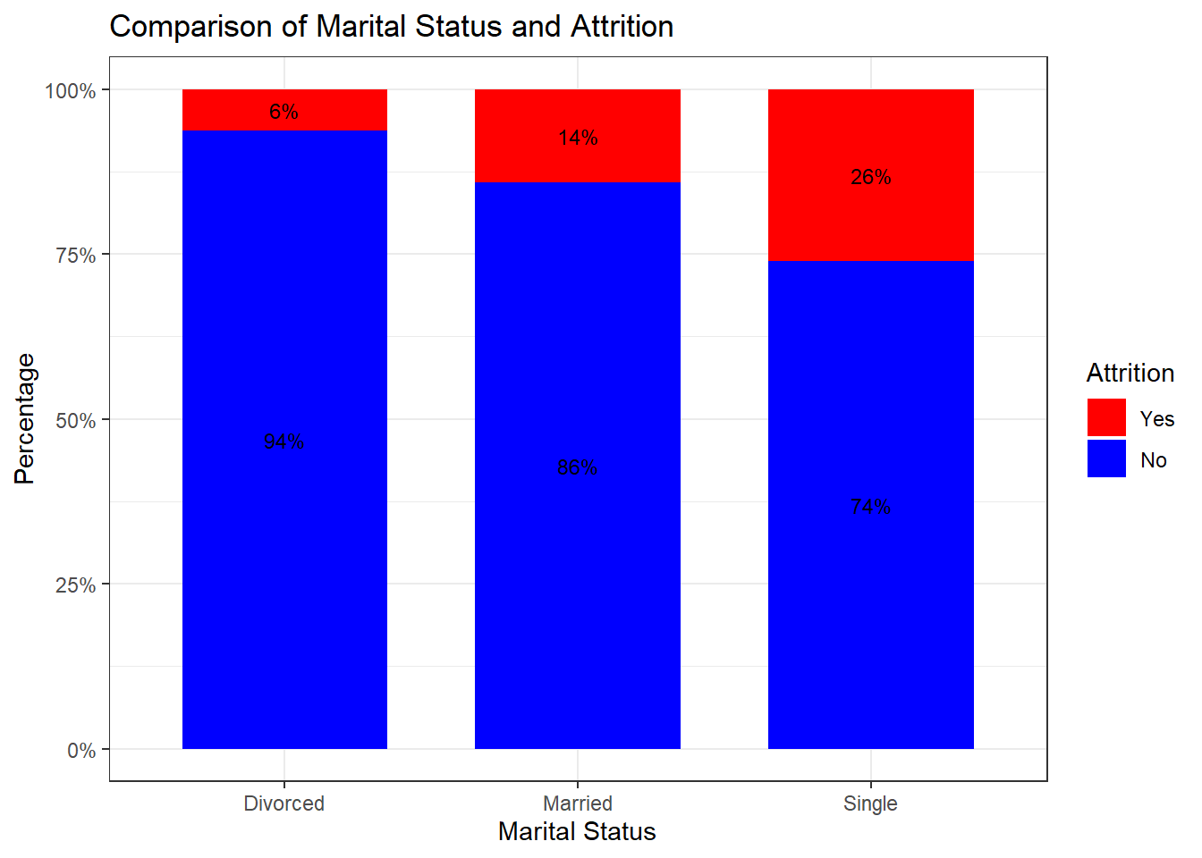
cordata <- attrition_Data %>%
   dplyr::select(c("DistanceFromHome", "MonthlyIncome",
                  "NumCompaniesWorked", "TotalWorkingYears",
                  "YearsAtCompany", "YearsInCurrentRole", "YearsSinceLastPromotion", "YearsWithCurrManager", "Age"))

# cordata <- attrition_Data %>%
#    dplyr::select(c("WorkLifeBalance", "MonthlyIncome",
#                   "OverTime", "JobRole",
#                    "YearsSinceLastPromotion", "Age"))


cormatrix <- cor(cordata)
round(cormatrix, 2)
## DistanceFromHome MonthlyIncome NumCompaniesWorked TotalWorkingYears YearsAtCompany YearsInCurrentRole YearsSinceLastPromotion YearsWithCurrManager
## DistanceFromHome 1.00 -0.01 -0.05 0.00 -0.02 -0.01 -0.02 -0.02
## MonthlyIncome -0.01 1.00 0.16 0.78 0.49 0.36 0.32 0.33
## NumCompaniesWorked -0.05 0.16 1.00 0.26 -0.14 -0.10 -0.07 -0.12
## TotalWorkingYears 0.00 0.78 0.26 1.00 0.64 0.49 0.45 0.46
## YearsAtCompany -0.02 0.49 -0.14 0.64 1.00 0.78 0.64 0.77
## YearsInCurrentRole -0.01 0.36 -0.10 0.49 0.78 1.00 0.55 0.71
## YearsSinceLastPromotion -0.02 0.32 -0.07 0.45 0.64 0.55 1.00 0.51
## YearsWithCurrManager -0.02 0.33 -0.12 0.46 0.77 0.71 0.51 1.00
## Age 0.01 0.48 0.29 0.65 0.29 0.21 0.22 0.19
## Age
## DistanceFromHome 0.01
## MonthlyIncome 0.48
## NumCompaniesWorked 0.29
## TotalWorkingYears 0.65
## YearsAtCompany 0.29
## YearsInCurrentRole 0.21
## YearsSinceLastPromotion 0.22
## YearsWithCurrManager 0.19
## Age 1.00ggcorrplot(cormatrix, hc.order = TRUE,outline.color = "white", lab = TRUE, colors = c("lightblue", "cornflowerblue", "blue"), lab_size = 2.5) +
labs(title="Correlation of Numeric Variables") 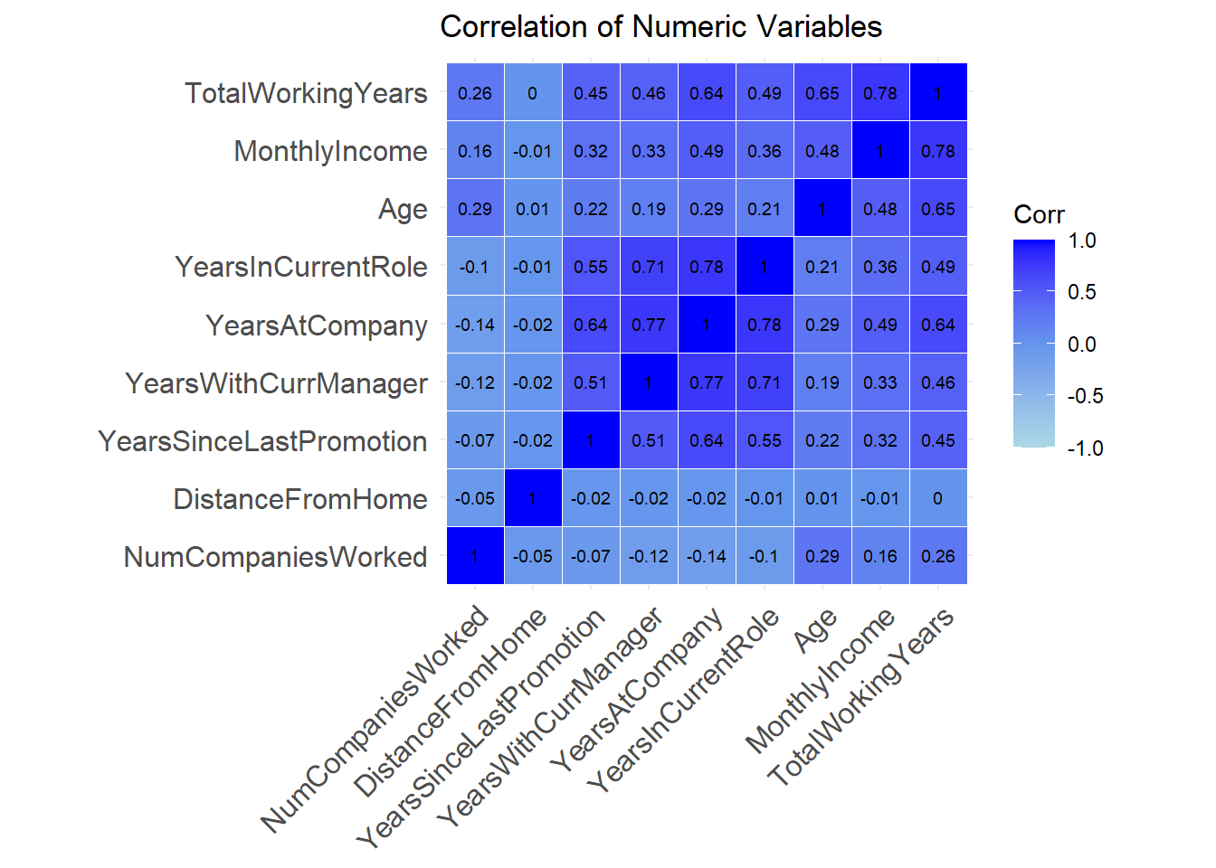
#define intercept-only model
intercept_only <- lm(Attrition ~ 1, data=attrition_Data3)

#define model with all predictors
attritionNum.lm <-glm(Attrition ~ Age + BusinessTravel + DailyRate + Department +
    DistanceFromHome + Education + EducationField + EmployeeNumber +
    EnvironmentSatisfaction + Gender + HourlyRate + JobInvolvement +
    JobLevel + JobRole + JobSatisfaction + MaritalStatus + MonthlyIncome +
    MonthlyRate + NumCompaniesWorked + OverTime + PercentSalaryHike +
    PerformanceRating + RelationshipSatisfaction + StockOptionLevel +
    TotalWorkingYears + TrainingTimesLastYear + WorkLifeBalance +
    YearsAtCompany + YearsInCurrentRole + YearsSinceLastPromotion +
    YearsWithCurrManager, data = attrition_Data3)


summary(attritionNum.lm)
##
## Call:
## glm(formula = Attrition ~ Age + BusinessTravel + DailyRate +
## Department + DistanceFromHome + Education + EducationField +
## EmployeeNumber + EnvironmentSatisfaction + Gender + HourlyRate +
## JobInvolvement + JobLevel + JobRole + JobSatisfaction + MaritalStatus +
## MonthlyIncome + MonthlyRate + NumCompaniesWorked + OverTime +
## PercentSalaryHike + PerformanceRating + RelationshipSatisfaction +
## StockOptionLevel + TotalWorkingYears + TrainingTimesLastYear +
## WorkLifeBalance + YearsAtCompany + YearsInCurrentRole + YearsSinceLastPromotion +
## YearsWithCurrManager, data = attrition_Data3)
##
## Coefficients:
## Estimate Std. Error t value Pr(>|t|)
## (Intercept) 7.117e-01 1.712e-01 4.157 3.55e-05 ***
## Age -3.542e-03 1.703e-03 -2.080 0.037870 *
## BusinessTravel 2.771e-04 1.658e-02 0.017 0.986668
## DailyRate -2.491e-05 2.770e-05 -0.900 0.368624
## Department -1.032e-01 2.592e-02 -3.979 7.51e-05 ***
## DistanceFromHome 3.745e-03 1.388e-03 2.699 0.007098 **
## Education -6.670e-03 1.126e-02 -0.592 0.553721
## EducationField 1.827e-02 8.609e-03 2.122 0.034151 *
## EmployeeNumber -9.959e-06 1.840e-05 -0.541 0.588540
## EnvironmentSatisfaction -2.858e-02 1.017e-02 -2.810 0.005063 **
## Gender -1.247e-02 2.258e-02 -0.552 0.580804
## HourlyRate 7.359e-04 5.546e-04 1.327 0.184898
## JobInvolvement -8.135e-02 1.590e-02 -5.115 3.89e-07 ***
## JobLevel -3.924e-02 3.551e-02 -1.105 0.269522
## JobRole 1.594e-02 5.045e-03 3.159 0.001640 **
## JobSatisfaction -4.091e-02 1.004e-02 -4.074 5.06e-05 ***
## MaritalStatus 1.052e-02 1.423e-02 0.739 0.460000
## MonthlyIncome 6.034e-06 8.202e-06 0.736 0.462144
## MonthlyRate -1.165e-06 1.568e-06 -0.743 0.457582
## NumCompaniesWorked 2.027e-02 5.080e-03 3.991 7.17e-05 ***
## OverTime 2.173e-01 2.455e-02 8.852 < 2e-16 ***
## PercentSalaryHike 1.335e-03 4.796e-03 0.278 0.780851
## PerformanceRating 1.015e-02 4.888e-02 0.208 0.835604
## RelationshipSatisfaction -2.222e-02 1.010e-02 -2.201 0.028035 *
## StockOptionLevel -5.115e-02 1.317e-02 -3.884 0.000111 ***
## TotalWorkingYears -6.168e-03 3.339e-03 -1.847 0.065111 .
## TrainingTimesLastYear -1.782e-02 8.774e-03 -2.030 0.042624 *
## WorkLifeBalance -3.772e-02 1.565e-02 -2.411 0.016142 *
## YearsAtCompany 4.687e-03 4.117e-03 1.139 0.255229
## YearsInCurrentRole -9.412e-03 5.146e-03 -1.829 0.067764 .
## YearsSinceLastPromotion 1.594e-02 4.607e-03 3.459 0.000569 ***
## YearsWithCurrManager -7.040e-03 5.057e-03 -1.392 0.164227
## ---
## Signif. codes: 0 '***' 0.001 '**' 0.01 '*' 0.05 '.' 0.1 ' ' 1
##
## (Dispersion parameter for gaussian family taken to be 0.1045281)
##
## Null deviance: 117.471 on 869 degrees of freedom
## Residual deviance: 87.595 on 838 degrees of freedom
## AIC: 537.63
##
## Number of Fisher Scoring iterations: 2#perform forward stepwise regression
model_forward <- step(intercept_only, direction='forward', scope=formula(attritionNum.lm), trace=FALSE)
summary(model_forward)##
## Call:
## lm(formula = Attrition ~ OverTime + JobInvolvement + TotalWorkingYears +
## JobSatisfaction + StockOptionLevel + NumCompaniesWorked +
## EnvironmentSatisfaction + YearsSinceLastPromotion + DistanceFromHome +
## YearsInCurrentRole + WorkLifeBalance + Age + RelationshipSatisfaction +
## Department + JobRole + EducationField + TrainingTimesLastYear +
## HourlyRate, data = attrition_Data3)
##
## Residuals:
## Min 1Q Median 3Q Max
## -0.64861 -0.20315 -0.08704 0.08022 1.11146
##
## Coefficients:
## Estimate Std. Error t value Pr(>|t|)
## (Intercept) 0.6799804 0.1123620 6.052 2.15e-09 ***
## OverTime 0.2195226 0.0243573 9.013 < 2e-16 ***
## JobInvolvement -0.0828589 0.0157415 -5.264 1.79e-07 ***
## TotalWorkingYears -0.0069995 0.0023021 -3.041 0.00243 **
## JobSatisfaction -0.0397962 0.0099250 -4.010 6.61e-05 ***
## StockOptionLevel -0.0527675 0.0129420 -4.077 4.99e-05 ***
## NumCompaniesWorked 0.0194493 0.0047889 4.061 5.33e-05 ***
## EnvironmentSatisfaction -0.0296318 0.0100677 -2.943 0.00334 **
## YearsSinceLastPromotion 0.0170840 0.0043050 3.968 7.85e-05 ***
## DistanceFromHome 0.0036809 0.0013601 2.706 0.00694 **
## YearsInCurrentRole -0.0097814 0.0039633 -2.468 0.01378 *
## WorkLifeBalance -0.0375746 0.0155476 -2.417 0.01587 *
## Age -0.0037222 0.0016622 -2.239 0.02540 *
## RelationshipSatisfaction -0.0219286 0.0099839 -2.196 0.02833 *
## Department -0.1007206 0.0255558 -3.941 8.77e-05 ***
## JobRole 0.0181787 0.0048312 3.763 0.00018 ***
## EducationField 0.0173904 0.0085329 2.038 0.04185 *
## TrainingTimesLastYear -0.0170907 0.0086991 -1.965 0.04978 *
## HourlyRate 0.0007780 0.0005501 1.414 0.15768
## ---
## Signif. codes: 0 '***' 0.001 '**' 0.01 '*' 0.05 '.' 0.1 ' ' 1
##
## Residual standard error: 0.3223 on 851 degrees of freedom
## Multiple R-squared: 0.2477, Adjusted R-squared: 0.2318
## F-statistic: 15.57 on 18 and 851 DF, p-value: < 2.2e-16#view results of forward stepwise regression
model_forward$anova#view final model
model_forward$coefficients## (Intercept) OverTime JobInvolvement TotalWorkingYears JobSatisfaction StockOptionLevel NumCompaniesWorked
## 0.679980353 0.219522581 -0.082858907 -0.006999530 -0.039796158 -0.052767487 0.019449320
## EnvironmentSatisfaction YearsSinceLastPromotion DistanceFromHome YearsInCurrentRole WorkLifeBalance Age RelationshipSatisfaction
## -0.029631794 0.017083996 0.003680928 -0.009781401 -0.037574553 -0.003722152 -0.021928593
## Department JobRole EducationField TrainingTimesLastYear HourlyRate
## -0.100720564 0.018178716 0.017390374 -0.017090726 0.000777976model_backward <- step(attritionNum.lm, direction = "backward", scope=formula(attritionNum.lm), trace = FALSE)
summary(model_backward)##
## Call:
## glm(formula = Attrition ~ Age + Department + DistanceFromHome +
## EducationField + EnvironmentSatisfaction + HourlyRate + JobInvolvement +
## JobRole + JobSatisfaction + NumCompaniesWorked + OverTime +
## RelationshipSatisfaction + StockOptionLevel + TotalWorkingYears +
## TrainingTimesLastYear + WorkLifeBalance + YearsInCurrentRole +
## YearsSinceLastPromotion, data = attrition_Data3)
##
## Coefficients:
## Estimate Std. Error t value Pr(>|t|)
## (Intercept) 0.6799804 0.1123620 6.052 2.15e-09 ***
## Age -0.0037222 0.0016622 -2.239 0.02540 *
## Department -0.1007206 0.0255558 -3.941 8.77e-05 ***
## DistanceFromHome 0.0036809 0.0013601 2.706 0.00694 **
## EducationField 0.0173904 0.0085329 2.038 0.04185 *
## EnvironmentSatisfaction -0.0296318 0.0100677 -2.943 0.00334 **
## HourlyRate 0.0007780 0.0005501 1.414 0.15768
## JobInvolvement -0.0828589 0.0157415 -5.264 1.79e-07 ***
## JobRole 0.0181787 0.0048312 3.763 0.00018 ***
## JobSatisfaction -0.0397962 0.0099250 -4.010 6.61e-05 ***
## NumCompaniesWorked 0.0194493 0.0047889 4.061 5.33e-05 ***
## OverTime 0.2195226 0.0243573 9.013 < 2e-16 ***
## RelationshipSatisfaction -0.0219286 0.0099839 -2.196 0.02833 *
## StockOptionLevel -0.0527675 0.0129420 -4.077 4.99e-05 ***
## TotalWorkingYears -0.0069995 0.0023021 -3.041 0.00243 **
## TrainingTimesLastYear -0.0170907 0.0086991 -1.965 0.04978 *
## WorkLifeBalance -0.0375746 0.0155476 -2.417 0.01587 *
## YearsInCurrentRole -0.0097814 0.0039633 -2.468 0.01378 *
## YearsSinceLastPromotion 0.0170840 0.0043050 3.968 7.85e-05 ***
## ---
## Signif. codes: 0 '***' 0.001 '**' 0.01 '*' 0.05 '.' 0.1 ' ' 1
##
## (Dispersion parameter for gaussian family taken to be 0.1038466)
##
## Null deviance: 117.471 on 869 degrees of freedom
## Residual deviance: 88.373 on 851 degrees of freedom
## AIC: 519.33
##
## Number of Fisher Scoring iterations: 2#view results of forward stepwise regression
model_backward$anova#view final model
model_backward$coefficients## (Intercept) Age Department DistanceFromHome EducationField EnvironmentSatisfaction HourlyRate
## 0.679980353 -0.003722152 -0.100720564 0.003680928 0.017390374 -0.029631794 0.000777976
## JobInvolvement JobRole JobSatisfaction NumCompaniesWorked OverTime RelationshipSatisfaction StockOptionLevel
## -0.082858907 0.018178716 -0.039796158 0.019449320 0.219522581 -0.021928593 -0.052767487
## TotalWorkingYears TrainingTimesLastYear WorkLifeBalance YearsInCurrentRole YearsSinceLastPromotion
## -0.006999530 -0.017090726 -0.037574553 -0.009781401 0.017083996model_both <- step(intercept_only, direction = "both", scope=formula(attritionNum.lm), trace = FALSE)
summary(model_both)##
## Call:
## lm(formula = Attrition ~ OverTime + JobInvolvement + TotalWorkingYears +
## JobSatisfaction + StockOptionLevel + NumCompaniesWorked +
## EnvironmentSatisfaction + YearsSinceLastPromotion + DistanceFromHome +
## YearsInCurrentRole + WorkLifeBalance + Age + RelationshipSatisfaction +
## Department + JobRole + EducationField + TrainingTimesLastYear +
## HourlyRate, data = attrition_Data3)
##
## Residuals:
## Min 1Q Median 3Q Max
## -0.64861 -0.20315 -0.08704 0.08022 1.11146
##
## Coefficients:
## Estimate Std. Error t value Pr(>|t|)
## (Intercept) 0.6799804 0.1123620 6.052 2.15e-09 ***
## OverTime 0.2195226 0.0243573 9.013 < 2e-16 ***
## JobInvolvement -0.0828589 0.0157415 -5.264 1.79e-07 ***
## TotalWorkingYears -0.0069995 0.0023021 -3.041 0.00243 **
## JobSatisfaction -0.0397962 0.0099250 -4.010 6.61e-05 ***
## StockOptionLevel -0.0527675 0.0129420 -4.077 4.99e-05 ***
## NumCompaniesWorked 0.0194493 0.0047889 4.061 5.33e-05 ***
## EnvironmentSatisfaction -0.0296318 0.0100677 -2.943 0.00334 **
## YearsSinceLastPromotion 0.0170840 0.0043050 3.968 7.85e-05 ***
## DistanceFromHome 0.0036809 0.0013601 2.706 0.00694 **
## YearsInCurrentRole -0.0097814 0.0039633 -2.468 0.01378 *
## WorkLifeBalance -0.0375746 0.0155476 -2.417 0.01587 *
## Age -0.0037222 0.0016622 -2.239 0.02540 *
## RelationshipSatisfaction -0.0219286 0.0099839 -2.196 0.02833 *
## Department -0.1007206 0.0255558 -3.941 8.77e-05 ***
## JobRole 0.0181787 0.0048312 3.763 0.00018 ***
## EducationField 0.0173904 0.0085329 2.038 0.04185 *
## TrainingTimesLastYear -0.0170907 0.0086991 -1.965 0.04978 *
## HourlyRate 0.0007780 0.0005501 1.414 0.15768
## ---
## Signif. codes: 0 '***' 0.001 '**' 0.01 '*' 0.05 '.' 0.1 ' ' 1
##
## Residual standard error: 0.3223 on 851 degrees of freedom
## Multiple R-squared: 0.2477, Adjusted R-squared: 0.2318
## F-statistic: 15.57 on 18 and 851 DF, p-value: < 2.2e-16#view results of forward stepwise regression
model_both$anova#view final model
model_both$coefficients## (Intercept) OverTime JobInvolvement TotalWorkingYears JobSatisfaction StockOptionLevel NumCompaniesWorked
## 0.679980353 0.219522581 -0.082858907 -0.006999530 -0.039796158 -0.052767487 0.019449320
## EnvironmentSatisfaction YearsSinceLastPromotion DistanceFromHome YearsInCurrentRole WorkLifeBalance Age RelationshipSatisfaction
## -0.029631794 0.017083996 0.003680928 -0.009781401 -0.037574553 -0.003722152 -0.021928593
## Department JobRole EducationField TrainingTimesLastYear HourlyRate
## -0.100720564 0.018178716 0.017390374 -0.017090726 0.000777976MaritalStatus + MonthlyIncome + PercentSalaryHike + PerformanceRating + YearsAtCompany + RelationshipSatisfaction + StockOptionLevel + TrainingTimesLastYear +
YearsInCurrentRole + YearsWithCurrManager + Age (none >60)+ EducationField + Department + EnvironmentSatisfaction + JobSatisfaction + TotalWorkingYears + MonthlyIncome +
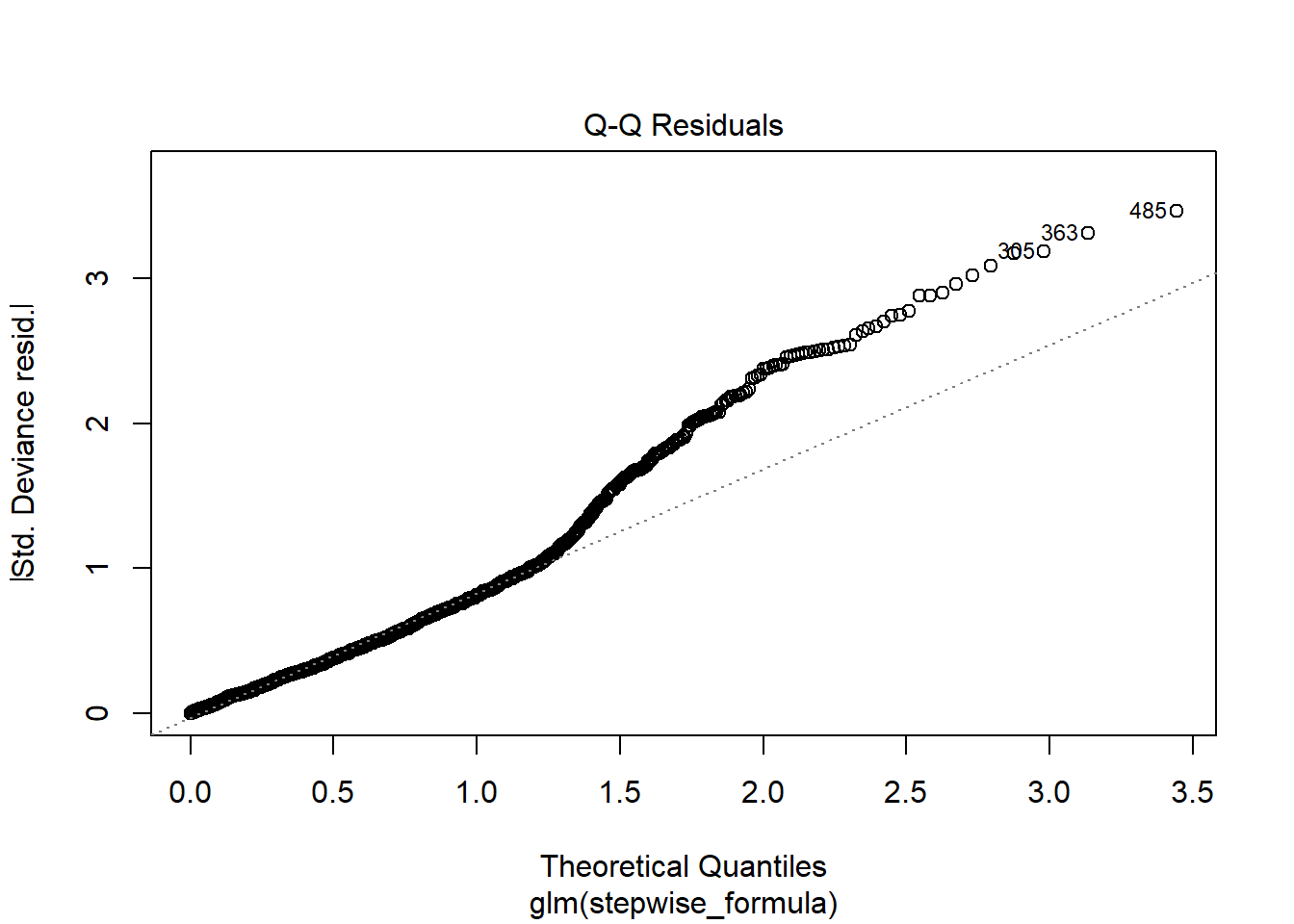
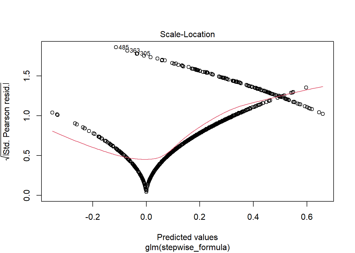
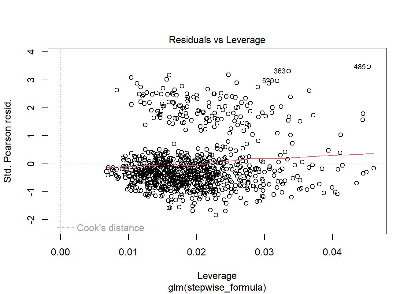
stepwise_formula <- Attrition ~ OverTime + JobRole + JobInvolvement + MaritalStatus +
    JobSatisfaction + WorkLifeBalance + NumCompaniesWorked + Age +  DistanceFromHome +
     EnvironmentSatisfaction + YearsSinceLastPromotion + YearsInCurrentRole +
  RelationshipSatisfaction + TrainingTimesLastYear + TotalWorkingYears  + BusinessTravel

#define model with all predictors
attritionNum.lm2 <-glm(stepwise_formula, data = attrition_Data3)


summary(attritionNum.lm2)
##
## Call:
## glm(formula = stepwise_formula, data = attrition_Data3)
##
## Coefficients:
## Estimate Std. Error t value Pr(>|t|)
## (Intercept) 0.6200672 0.1132177 5.477 5.70e-08 ***
## OverTime 0.2179106 0.0248866 8.756 < 2e-16 ***
## JobRole 0.0070621 0.0040217 1.756 0.079444 .
## JobInvolvement -0.0914259 0.0159509 -5.732 1.38e-08 ***
## MaritalStatus 0.0188943 0.0142773 1.323 0.186065
## JobSatisfaction -0.0419333 0.0100980 -4.153 3.62e-05 ***
## WorkLifeBalance -0.0387398 0.0158246 -2.448 0.014562 *
## NumCompaniesWorked 0.0181884 0.0048842 3.724 0.000209 ***
## Age -0.0042818 0.0016918 -2.531 0.011555 *
## DistanceFromHome 0.0031438 0.0013898 2.262 0.023939 *
## EnvironmentSatisfaction -0.0309287 0.0102442 -3.019 0.002610 **
## YearsSinceLastPromotion 0.0182855 0.0043946 4.161 3.49e-05 ***
## YearsInCurrentRole -0.0116864 0.0040346 -2.897 0.003870 **
## RelationshipSatisfaction -0.0192751 0.0101991 -1.890 0.059113 .
## TrainingTimesLastYear -0.0147434 0.0088560 -1.665 0.096321 .
## TotalWorkingYears -0.0071340 0.0023489 -3.037 0.002460 **
## BusinessTravel 0.0002016 0.0167468 0.012 0.990397
## ---
## Signif. codes: 0 '***' 0.001 '**' 0.01 '*' 0.05 '.' 0.1 ' ' 1
##
## (Dispersion parameter for gaussian family taken to be 0.1081266)
##
## Null deviance: 117.471 on 869 degrees of freedom
## Residual deviance: 92.232 on 853 degrees of freedom
## AIC: 552.51
##
## Number of Fisher Scoring iterations: 2plot(attritionNum.lm2)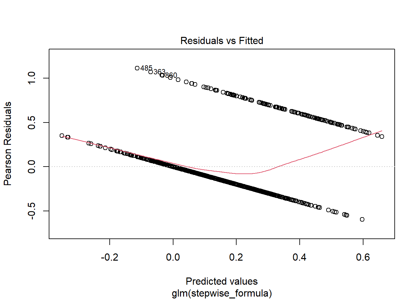
cordata <- attrition_Data3 %>%
   dplyr::select(c("OverTime", "JobRole", "JobInvolvement", "MaritalStatus",
    "JobSatisfaction",  "WorkLifeBalance", "NumCompaniesWorked", "Age", "DistanceFromHome",
     "EnvironmentSatisfaction", "YearsSinceLastPromotion", "YearsInCurrentRole",
  "RelationshipSatisfaction", "TrainingTimesLastYear", "TotalWorkingYears", "BusinessTravel"))

# cordata <- attrition_Data %>%
#    dplyr::select(c("WorkLifeBalance", "MonthlyIncome",
#                   "OverTime", "JobRole",
#                    "YearsSinceLastPromotion", "Age"))


cormatrix <- cor(cordata)
round(cormatrix, 2)
## OverTime JobRole JobInvolvement MaritalStatus JobSatisfaction WorkLifeBalance NumCompaniesWorked Age DistanceFromHome EnvironmentSatisfaction
## OverTime 1.00 -0.07 -0.04 -0.04 0.03 0.00 0.00 0.00 0.06 0.06
## JobRole -0.07 1.00 -0.03 0.03 -0.01 -0.03 -0.04 -0.07 -0.02 0.04
## JobInvolvement -0.04 -0.03 1.00 -0.02 -0.05 0.01 -0.01 0.02 0.00 0.00
## MaritalStatus -0.04 0.03 -0.02 1.00 0.00 -0.02 0.01 0.03 0.08 -0.04
## JobSatisfaction 0.03 -0.01 -0.05 0.00 1.00 -0.03 -0.08 -0.02 -0.02 -0.02
## WorkLifeBalance 0.00 -0.03 0.01 -0.02 -0.03 1.00 0.02 -0.01 -0.01 0.08
## NumCompaniesWorked 0.00 -0.04 -0.01 0.01 -0.08 0.02 1.00 0.29 -0.05 0.01
## Age 0.00 -0.07 0.02 0.03 -0.02 -0.01 0.29 1.00 0.01 -0.01
## DistanceFromHome 0.06 -0.02 0.00 0.08 -0.02 -0.01 -0.05 0.01 1.00 -0.04
## EnvironmentSatisfaction 0.06 0.04 0.00 -0.04 -0.02 0.08 0.01 -0.01 -0.04 1.00
## YearsSinceLastPromotion -0.02 -0.06 -0.03 0.04 -0.02 0.04 -0.07 0.22 -0.02 0.01
## YearsInCurrentRole -0.03 -0.13 0.01 0.06 0.00 0.08 -0.10 0.21 -0.01 0.02
## RelationshipSatisfaction 0.02 0.03 0.02 -0.05 -0.03 0.04 0.04 -0.01 0.04 0.00
## TrainingTimesLastYear -0.06 0.07 -0.02 -0.04 -0.03 0.02 -0.07 -0.05 -0.04 -0.01
## TotalWorkingYears -0.03 -0.11 -0.01 0.04 -0.05 0.02 0.26 0.65 0.00 -0.02
## BusinessTravel -0.03 -0.02 -0.04 -0.08 0.04 0.03 0.02 0.00 0.06 0.00
## YearsSinceLastPromotion YearsInCurrentRole RelationshipSatisfaction TrainingTimesLastYear TotalWorkingYears BusinessTravel
## OverTime -0.02 -0.03 0.02 -0.06 -0.03 -0.03
## JobRole -0.06 -0.13 0.03 0.07 -0.11 -0.02
## JobInvolvement -0.03 0.01 0.02 -0.02 -0.01 -0.04
## MaritalStatus 0.04 0.06 -0.05 -0.04 0.04 -0.08
## JobSatisfaction -0.02 0.00 -0.03 -0.03 -0.05 0.04
## WorkLifeBalance 0.04 0.08 0.04 0.02 0.02 0.03
## NumCompaniesWorked -0.07 -0.10 0.04 -0.07 0.26 0.02
## Age 0.22 0.21 -0.01 -0.05 0.65 0.00
## DistanceFromHome -0.02 -0.01 0.04 -0.04 0.00 0.06
## EnvironmentSatisfaction 0.01 0.02 0.00 -0.01 -0.02 0.00
## YearsSinceLastPromotion 1.00 0.55 0.03 -0.04 0.45 0.04
## YearsInCurrentRole 0.55 1.00 0.00 -0.02 0.49 -0.02
## RelationshipSatisfaction 0.03 0.00 1.00 0.02 -0.02 0.05
## TrainingTimesLastYear -0.04 -0.02 0.02 1.00 -0.04 0.00
## TotalWorkingYears 0.45 0.49 -0.02 -0.04 1.00 -0.03
## BusinessTravel 0.04 -0.02 0.05 0.00 -0.03 1.00ggcorrplot(cormatrix, hc.order = TRUE,outline.color = "white", lab = TRUE, colors = c("lightblue", "cornflowerblue", "blue"), lab_size = 2.5) +
labs(title="Correlation of Numeric Variables") 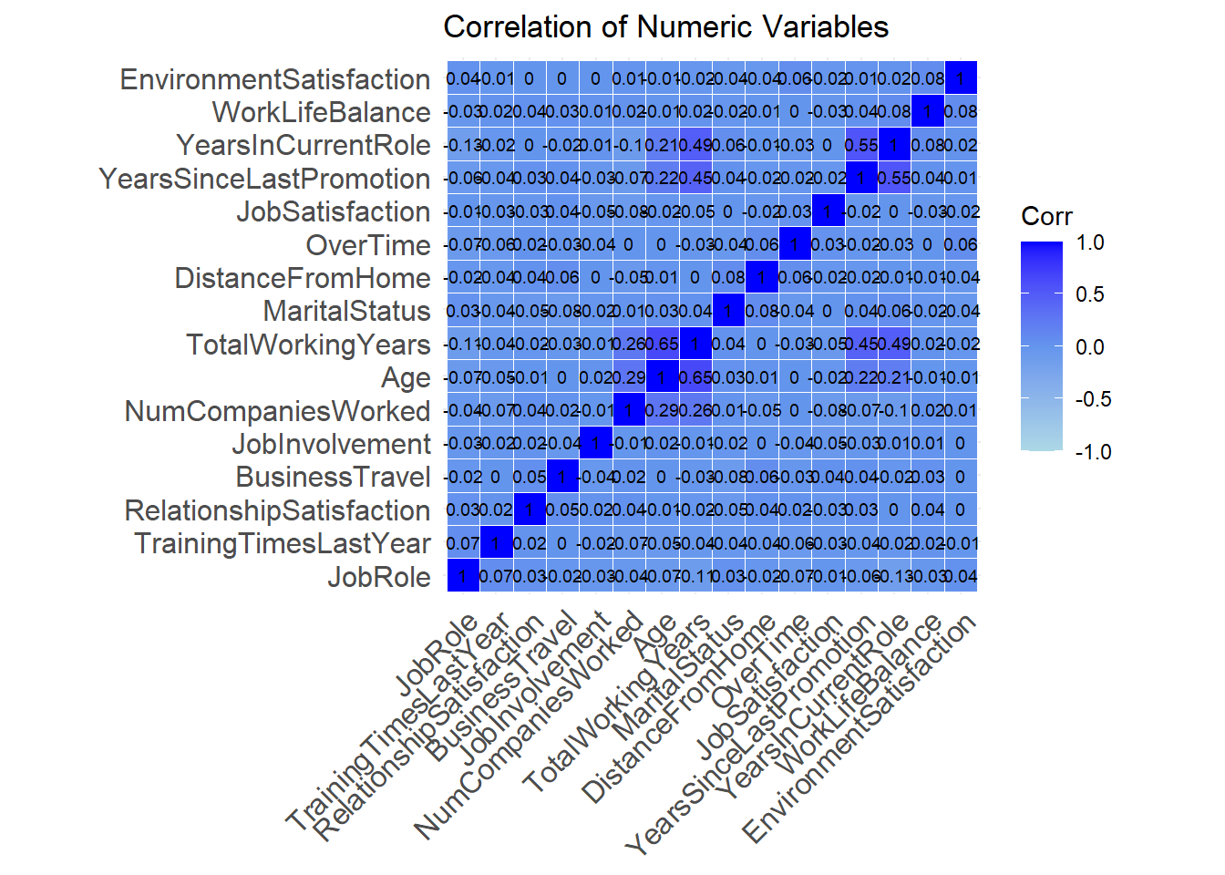
# The results of the stepwise analysis
stepwise_formula <- Attrition ~ OverTime + JobRole + JobInvolvement + MaritalStatus +
    JobSatisfaction + WorkLifeBalance + NumCompaniesWorked + Age +  DistanceFromHome +
     EnvironmentSatisfaction + YearsSinceLastPromotion + YearsInCurrentRole +
  RelationshipSatisfaction + TrainingTimesLastYear + TotalWorkingYears  + BusinessTravel

stepwise_formula2 <- Attrition ~ OverTime + JobInvolvement +
    JobSatisfaction + NumCompaniesWorked + Age +
     EnvironmentSatisfaction + YearsSinceLastPromotion + TotalWorkingYears

# Create the first test model
model_test <- glm(Attrition~., attrition_Data3, family = "binomial")

summary(model_test)
##
## Call:
## glm(formula = Attrition ~ ., family = "binomial", data = attrition_Data3)
##
## Coefficients:
## Estimate Std. Error z value Pr(>|z|)
## (Intercept) 3.334e+00 1.782e+00 1.871 0.061330 .
## ID 2.552e-04 4.709e-04 0.542 0.587915
## Age -2.924e-02 1.761e-02 -1.660 0.096820 .
## BusinessTravel -7.116e-02 1.761e-01 -0.404 0.686215
## DailyRate -2.866e-04 2.898e-04 -0.989 0.322644
## Department -1.224e+00 2.835e-01 -4.317 1.58e-05 ***
## DistanceFromHome 4.245e-02 1.434e-02 2.960 0.003078 **
## Education -1.046e-02 1.166e-01 -0.090 0.928535
## EducationField 1.715e-01 8.977e-02 1.910 0.056098 .
## EmployeeNumber -4.039e-05 1.909e-04 -0.212 0.832472
## EnvironmentSatisfaction -3.272e-01 1.082e-01 -3.024 0.002494 **
## Gender -1.754e-01 2.384e-01 -0.736 0.461777
## HourlyRate 9.831e-03 5.889e-03 1.669 0.095067 .
## JobInvolvement -7.243e-01 1.622e-01 -4.465 8.01e-06 ***
## JobLevel -2.301e-01 3.928e-01 -0.586 0.558067
## JobRole 1.937e-01 5.264e-02 3.681 0.000233 ***
## JobSatisfaction -3.914e-01 1.049e-01 -3.732 0.000190 ***
## MaritalStatus 1.363e-01 1.625e-01 0.839 0.401456
## MonthlyIncome -1.703e-06 9.225e-05 -0.018 0.985272
## MonthlyRate -1.409e-05 1.672e-05 -0.843 0.399462
## NumCompaniesWorked 2.224e-01 5.009e-02 4.441 8.97e-06 ***
## OverTime 1.921e+00 2.428e-01 7.912 2.54e-15 ***
## PercentSalaryHike -2.277e-02 5.077e-02 -0.449 0.653743
## PerformanceRating 2.550e-01 5.149e-01 0.495 0.620382
## RelationshipSatisfaction -2.236e-01 1.045e-01 -2.139 0.032423 *
## StockOptionLevel -6.003e-01 1.554e-01 -3.862 0.000112 ***
## TotalWorkingYears -9.568e-02 3.879e-02 -2.467 0.013640 *
## TrainingTimesLastYear -2.259e-01 9.566e-02 -2.361 0.018219 *
## WorkLifeBalance -4.222e-01 1.575e-01 -2.680 0.007362 **
## YearsAtCompany 8.165e-02 4.957e-02 1.647 0.099516 .
## YearsInCurrentRole -1.382e-01 5.795e-02 -2.384 0.017108 *
## YearsSinceLastPromotion 2.355e-01 5.620e-02 4.191 2.78e-05 ***
## YearsWithCurrManager -1.271e-01 5.890e-02 -2.157 0.030992 *
## ---
## Signif. codes: 0 '***' 0.001 '**' 0.01 '*' 0.05 '.' 0.1 ' ' 1
##
## (Dispersion parameter for binomial family taken to be 1)
##
## Null deviance: 767.67 on 869 degrees of freedom
## Residual deviance: 509.68 on 837 degrees of freedom
## AIC: 575.68
##
## Number of Fisher Scoring iterations: 6# Locking Random
RNGkind(sample.kind = "Rounding")## Warning in RNGkind(sample.kind = "Rounding"): non-uniform 'Rounding' sampler usedset.seed(9170) #4170
# Index
index <- sample(nrow(attrition_Data3), nrow(attrition_Data3)*0.7)
# Splitting
training_set_att <- attrition_Data3[index,]
testing_set_att <- attrition_Data3[-index,]
#--------------------------------------------------------
model_base <- glm(Attrition~., training_set_att, family = "binomial")
summary(model_base)##
## Call:
## glm(formula = Attrition ~ ., family = "binomial", data = training_set_att)
##
## Coefficients:
## Estimate Std. Error z value Pr(>|z|)
## (Intercept) 1.801e+00 2.164e+00 0.832 0.405306
## ID 4.207e-04 5.737e-04 0.733 0.463449
## Age -1.115e-02 2.082e-02 -0.536 0.592222
## BusinessTravel 6.955e-02 2.159e-01 0.322 0.747359
## DailyRate -8.545e-04 3.663e-04 -2.333 0.019660 *
## Department -1.301e+00 3.460e-01 -3.760 0.000170 ***
## DistanceFromHome 3.820e-02 1.817e-02 2.103 0.035499 *
## Education -1.193e-01 1.451e-01 -0.822 0.411095
## EducationField 2.058e-01 1.111e-01 1.852 0.063973 .
## EmployeeNumber 3.404e-05 2.288e-04 0.149 0.881753
## EnvironmentSatisfaction -3.411e-01 1.346e-01 -2.535 0.011236 *
## Gender -2.511e-01 2.883e-01 -0.871 0.383763
## HourlyRate 1.511e-02 7.155e-03 2.112 0.034729 *
## JobInvolvement -6.712e-01 1.987e-01 -3.379 0.000728 ***
## JobLevel -7.382e-01 4.689e-01 -1.574 0.115402
## JobRole 1.775e-01 6.253e-02 2.838 0.004537 **
## JobSatisfaction -4.390e-01 1.285e-01 -3.417 0.000634 ***
## MaritalStatus 3.347e-01 2.027e-01 1.651 0.098683 .
## MonthlyIncome 1.649e-04 1.108e-04 1.488 0.136662
## MonthlyRate -1.004e-05 2.030e-05 -0.495 0.620875
## NumCompaniesWorked 2.659e-01 6.112e-02 4.350 1.36e-05 ***
## OverTime 2.076e+00 3.119e-01 6.656 2.80e-11 ***
## PercentSalaryHike -4.552e-02 6.150e-02 -0.740 0.459165
## PerformanceRating 4.967e-01 6.360e-01 0.781 0.434858
## RelationshipSatisfaction -1.570e-01 1.283e-01 -1.224 0.221132
## StockOptionLevel -7.173e-01 1.893e-01 -3.789 0.000151 ***
## TotalWorkingYears -1.279e-01 4.437e-02 -2.882 0.003953 **
## TrainingTimesLastYear -2.767e-01 1.141e-01 -2.424 0.015336 *
## WorkLifeBalance -3.047e-01 2.002e-01 -1.522 0.128010
## YearsAtCompany 3.019e-02 5.814e-02 0.519 0.603587
## YearsInCurrentRole -1.130e-01 6.781e-02 -1.666 0.095673 .
## YearsSinceLastPromotion 2.604e-01 6.793e-02 3.833 0.000126 ***
## YearsWithCurrManager -8.480e-02 6.808e-02 -1.246 0.212904
## ---
## Signif. codes: 0 '***' 0.001 '**' 0.01 '*' 0.05 '.' 0.1 ' ' 1
##
## (Dispersion parameter for binomial family taken to be 1)
##
## Null deviance: 543.93 on 608 degrees of freedom
## Residual deviance: 354.24 on 576 degrees of freedom
## AIC: 420.24
##
## Number of Fisher Scoring iterations: 6#-------------------------------------------------------
model_sig <- glm(stepwise_formula, training_set_att, family = "binomial")
summary(model_sig)##
## Call:
## glm(formula = stepwise_formula, family = "binomial", data = training_set_att)
##
## Coefficients:
## Estimate Std. Error z value Pr(>|z|)
## (Intercept) 1.59571 1.22615 1.301 0.193123
## OverTime 1.73630 0.27372 6.343 2.25e-10 ***
## JobRole 0.05030 0.04672 1.077 0.281650
## JobInvolvement -0.72286 0.18098 -3.994 6.49e-05 ***
## MaritalStatus 0.26560 0.17334 1.532 0.125451
## JobSatisfaction -0.44459 0.11819 -3.762 0.000169 ***
## WorkLifeBalance -0.24537 0.17709 -1.386 0.165889
## NumCompaniesWorked 0.19644 0.05329 3.686 0.000227 ***
## Age -0.02435 0.01908 -1.276 0.201872
## DistanceFromHome 0.01422 0.01572 0.904 0.365753
## EnvironmentSatisfaction -0.29035 0.11919 -2.436 0.014845 *
## YearsSinceLastPromotion 0.25219 0.05638 4.473 7.71e-06 ***
## YearsInCurrentRole -0.14672 0.05432 -2.701 0.006917 **
## RelationshipSatisfaction -0.11125 0.11854 -0.938 0.347998
## TrainingTimesLastYear -0.19440 0.10478 -1.855 0.063548 .
## TotalWorkingYears -0.11268 0.03160 -3.566 0.000363 ***
## BusinessTravel 0.05072 0.19244 0.264 0.792121
## ---
## Signif. codes: 0 '***' 0.001 '**' 0.01 '*' 0.05 '.' 0.1 ' ' 1
##
## (Dispersion parameter for binomial family taken to be 1)
##
## Null deviance: 543.93 on 608 degrees of freedom
## Residual deviance: 402.73 on 592 degrees of freedom
## AIC: 436.73
##
## Number of Fisher Scoring iterations: 6#-----------------------------------------------------
# model_step <- step(model_base, direction = "backward", trace = FALSE)
#
# summary(model_step)
model_step <- step(intercept_only, direction = "both", scope=formula(stepwise_formula), trace = FALSE)
summary(model_step)##
## Call:
## lm(formula = Attrition ~ OverTime + JobInvolvement + TotalWorkingYears +
## JobSatisfaction + EnvironmentSatisfaction + NumCompaniesWorked +
## YearsSinceLastPromotion + YearsInCurrentRole + WorkLifeBalance +
## Age + DistanceFromHome + RelationshipSatisfaction + JobRole +
## TrainingTimesLastYear, data = attrition_Data3)
##
## Residuals:
## Min 1Q Median 3Q Max
## -0.58552 -0.20991 -0.08656 0.05677 1.12396
##
## Coefficients:
## Estimate Std. Error t value Pr(>|t|)
## (Intercept) 0.666458 0.104941 6.351 3.48e-10 ***
## OverTime 0.216590 0.024837 8.720 < 2e-16 ***
## JobInvolvement -0.091850 0.015931 -5.765 1.14e-08 ***
## TotalWorkingYears -0.007167 0.002344 -3.058 0.002295 **
## JobSatisfaction -0.041864 0.010086 -4.151 3.65e-05 ***
## EnvironmentSatisfaction -0.031468 0.010235 -3.075 0.002174 **
## NumCompaniesWorked 0.018310 0.004879 3.753 0.000187 ***
## YearsSinceLastPromotion 0.018346 0.004380 4.188 3.10e-05 ***
## YearsInCurrentRole -0.011414 0.004028 -2.834 0.004711 **
## WorkLifeBalance -0.039068 0.015816 -2.470 0.013700 *
## Age -0.004254 0.001691 -2.516 0.012057 *
## DistanceFromHome 0.003307 0.001380 2.396 0.016807 *
## RelationshipSatisfaction -0.020040 0.010174 -1.970 0.049195 *
## JobRole 0.007292 0.004017 1.816 0.069785 .
## TrainingTimesLastYear -0.015197 0.008848 -1.718 0.086234 .
## ---
## Signif. codes: 0 '***' 0.001 '**' 0.01 '*' 0.05 '.' 0.1 ' ' 1
##
## Residual standard error: 0.3288 on 855 degrees of freedom
## Multiple R-squared: 0.2132, Adjusted R-squared: 0.2004
## F-statistic: 16.55 on 14 and 855 DF, p-value: < 2.2e-16#------------------Predicting the model---------------------------------
# Predict model base
testing_set_att$pred_att_bs <- predict(model_base, newdata = testing_set_att, type = "response")
# Predict significant only model
testing_set_att$pred_att_sig <- predict(model_sig, newdata = testing_set_att, type = "response")
# Predict step wise model
testing_set_att$pred_att_stp <- predict(model_step, newdata = testing_set_att, type = "response")
#------------------Changing odds to labels-----------------------------------------------------
# Label model base
testing_set_att$label_bs <- ifelse(testing_set_att$pred_att_bs>0.5, 1, 0)
# Label model sig
testing_set_att$label_sig <- ifelse(testing_set_att$pred_att_sig>0.5, 1, 0)
# Label model step
testing_set_att$label_stp <- ifelse(testing_set_att$pred_att_stp>0.5, 1, 0)naive_ea <- naiveBayes(Attrition~., training_set_att, laplace = 1)
testing_set_att$pred_nv <- predict(object = naive_ea,
newdata = testing_set_att %>% dplyr::select(-c(pred_att_bs, pred_att_sig, pred_att_stp, label_bs,
label_sig, label_stp)),
type="class")
confusionMatrix(data = as.factor(testing_set_att$pred_nv), reference = as.factor(testing_set_att$Attrition), positive = "1")## Confusion Matrix and Statistics
##
## Reference
## Prediction 0 1
## 0 189 12
## 1 32 28
##
## Accuracy : 0.8314
## 95% CI : (0.7804, 0.8748)
## No Information Rate : 0.8467
## P-Value [Acc > NIR] : 0.782690
##
## Kappa : 0.4608
##
## Mcnemar's Test P-Value : 0.004179
##
## Sensitivity : 0.7000
## Specificity : 0.8552
## Pos Pred Value : 0.4667
## Neg Pred Value : 0.9403
## Prevalence : 0.1533
## Detection Rate : 0.1073
## Detection Prevalence : 0.2299
## Balanced Accuracy : 0.7776
##
## 'Positive' Class : 1
## stepWiseResult <- c( "OverTime", "JobRole", "JobInvolvement", "MaritalStatus",
"JobSatisfaction", "WorkLifeBalance", "NumCompaniesWorked", "Age", "DistanceFromHome",
"EnvironmentSatisfaction", "YearsSinceLastPromotion", "YearsInCurrentRole",
"RelationshipSatisfaction", "TrainingTimesLastYear", "TotalWorkingYears", "BusinessTravel")
# Use KNN to classify attrition in the testing set
classifications_att <- knn(train = training_set_att[, stepWiseResult],
test = testing_set_att[, stepWiseResult],
cl = training_set_att$Attrition, prob = TRUE, k = 5)
# Make sure 'classifications' and 'testing_set$Survived' have the same length
if (length(classifications_att) != nrow(testing_set_att)) {
stop("Mismatch in the length of 'classifications' and 'training_set_att$Attrition'")
}
# Create a table to compare the predicted classes with the actual classes
class_table_att <- table(classifications_att, testing_set_att$Attrition)
# Calculate and print the confusion matrix
confusion_matrix_att <- confusionMatrix(class_table_att)
confusion_matrix_att## Confusion Matrix and Statistics
##
##
## classifications_att 0 1
## 0 217 33
## 1 4 7
##
## Accuracy : 0.8582
## 95% CI : (0.8099, 0.8982)
## No Information Rate : 0.8467
## P-Value [Acc > NIR] : 0.3398
##
## Kappa : 0.2232
##
## Mcnemar's Test P-Value : 4.161e-06
##
## Sensitivity : 0.9819
## Specificity : 0.1750
## Pos Pred Value : 0.8680
## Neg Pred Value : 0.6364
## Prevalence : 0.8467
## Detection Rate : 0.8314
## Detection Prevalence : 0.9579
## Balanced Accuracy : 0.5785
##
## 'Positive' Class : 0
## get the average of the test sets
Loop for many k and the average of many training / test partition
iterations = 500
numks = 30
masterAcc = matrix(nrow = iterations, ncol = numks)
for(j in 1:iterations)
{
accs = data.frame(accuracy = numeric(30), k = numeric(30))
# Index
index <- sample(nrow(attrition_Data3), nrow(attrition_Data3)*0.7)
# Splitting
training_set_att <- attrition_Data3[index,]
testing_set_att <- attrition_Data3[-index,]
for(i in 1:30)
{
classifications_att <- knn(train = training_set_att[, stepWiseResult],
test = testing_set_att[, stepWiseResult],
cl = training_set_att$Attrition, prob = TRUE, k = i)
class_table = table(classifications_att, testing_set_att$Attrition)
CM = confusionMatrix(class_table)
masterAcc[j,i] = CM$overall[1]
}
}
MeanAcc = colMeans(masterAcc)
plot(seq(1,numks,1),MeanAcc, type = "l")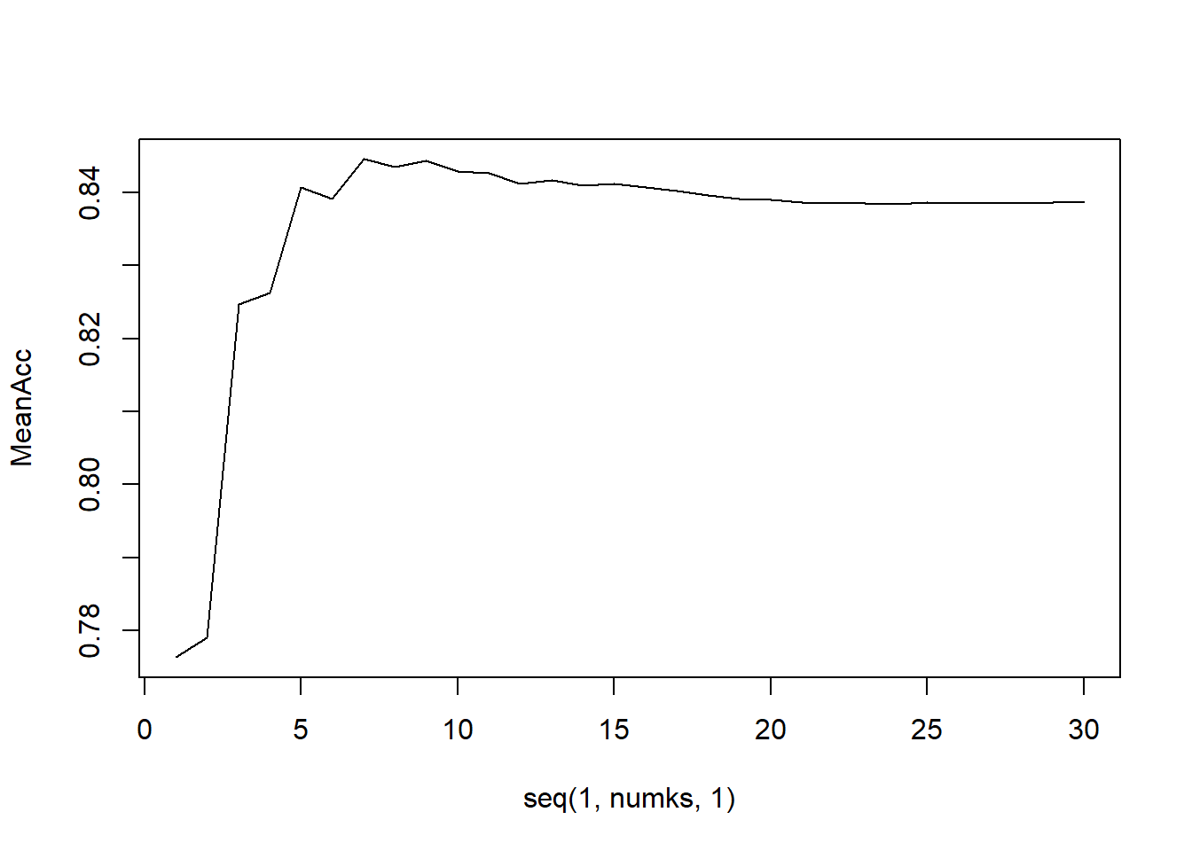
# Locking Random
RNGkind(sample.kind = "Rounding")
## Warning in RNGkind(sample.kind = "Rounding"): non-uniform 'Rounding' sampler usedset.seed(9170)
# Splitting
training_set_att <- attrition_Data3
testing_set_att2 <- attrition_Data_no_attrition
#--------------------------------------------------------
model_base <- glm(Attrition~., training_set_att, family = "binomial")
summary(model_base)##
## Call:
## glm(formula = Attrition ~ ., family = "binomial", data = training_set_att)
##
## Coefficients:
## Estimate Std. Error z value Pr(>|z|)
## (Intercept) 3.334e+00 1.782e+00 1.871 0.061330 .
## ID 2.552e-04 4.709e-04 0.542 0.587915
## Age -2.924e-02 1.761e-02 -1.660 0.096820 .
## BusinessTravel -7.116e-02 1.761e-01 -0.404 0.686215
## DailyRate -2.866e-04 2.898e-04 -0.989 0.322644
## Department -1.224e+00 2.835e-01 -4.317 1.58e-05 ***
## DistanceFromHome 4.245e-02 1.434e-02 2.960 0.003078 **
## Education -1.046e-02 1.166e-01 -0.090 0.928535
## EducationField 1.715e-01 8.977e-02 1.910 0.056098 .
## EmployeeNumber -4.039e-05 1.909e-04 -0.212 0.832472
## EnvironmentSatisfaction -3.272e-01 1.082e-01 -3.024 0.002494 **
## Gender -1.754e-01 2.384e-01 -0.736 0.461777
## HourlyRate 9.831e-03 5.889e-03 1.669 0.095067 .
## JobInvolvement -7.243e-01 1.622e-01 -4.465 8.01e-06 ***
## JobLevel -2.301e-01 3.928e-01 -0.586 0.558067
## JobRole 1.937e-01 5.264e-02 3.681 0.000233 ***
## JobSatisfaction -3.914e-01 1.049e-01 -3.732 0.000190 ***
## MaritalStatus 1.363e-01 1.625e-01 0.839 0.401456
## MonthlyIncome -1.703e-06 9.225e-05 -0.018 0.985272
## MonthlyRate -1.409e-05 1.672e-05 -0.843 0.399462
## NumCompaniesWorked 2.224e-01 5.009e-02 4.441 8.97e-06 ***
## OverTime 1.921e+00 2.428e-01 7.912 2.54e-15 ***
## PercentSalaryHike -2.277e-02 5.077e-02 -0.449 0.653743
## PerformanceRating 2.550e-01 5.149e-01 0.495 0.620382
## RelationshipSatisfaction -2.236e-01 1.045e-01 -2.139 0.032423 *
## StockOptionLevel -6.003e-01 1.554e-01 -3.862 0.000112 ***
## TotalWorkingYears -9.568e-02 3.879e-02 -2.467 0.013640 *
## TrainingTimesLastYear -2.259e-01 9.566e-02 -2.361 0.018219 *
## WorkLifeBalance -4.222e-01 1.575e-01 -2.680 0.007362 **
## YearsAtCompany 8.165e-02 4.957e-02 1.647 0.099516 .
## YearsInCurrentRole -1.382e-01 5.795e-02 -2.384 0.017108 *
## YearsSinceLastPromotion 2.355e-01 5.620e-02 4.191 2.78e-05 ***
## YearsWithCurrManager -1.271e-01 5.890e-02 -2.157 0.030992 *
## ---
## Signif. codes: 0 '***' 0.001 '**' 0.01 '*' 0.05 '.' 0.1 ' ' 1
##
## (Dispersion parameter for binomial family taken to be 1)
##
## Null deviance: 767.67 on 869 degrees of freedom
## Residual deviance: 509.68 on 837 degrees of freedom
## AIC: 575.68
##
## Number of Fisher Scoring iterations: 6#-------------------------------------------------------
model_sig <- glm(stepwise_formula, training_set_att, family = "binomial")
summary(model_sig)##
## Call:
## glm(formula = stepwise_formula, family = "binomial", data = training_set_att)
##
## Coefficients:
## Estimate Std. Error z value Pr(>|z|)
## (Intercept) 2.58977 1.05541 2.454 0.014136 *
## OverTime 1.75734 0.22617 7.770 7.85e-15 ***
## JobRole 0.06984 0.03964 1.762 0.078122 .
## JobInvolvement -0.79939 0.15123 -5.286 1.25e-07 ***
## MaritalStatus 0.16561 0.14357 1.154 0.248691
## JobSatisfaction -0.41111 0.09934 -4.138 3.50e-05 ***
## WorkLifeBalance -0.38114 0.14626 -2.606 0.009165 **
## NumCompaniesWorked 0.18055 0.04486 4.024 5.71e-05 ***
## Age -0.03592 0.01658 -2.166 0.030293 *
## DistanceFromHome 0.02870 0.01301 2.206 0.027392 *
## EnvironmentSatisfaction -0.30105 0.10011 -3.007 0.002636 **
## YearsSinceLastPromotion 0.23679 0.04810 4.923 8.52e-07 ***
## YearsInCurrentRole -0.15033 0.04601 -3.267 0.001086 **
## RelationshipSatisfaction -0.17954 0.09840 -1.825 0.068053 .
## TrainingTimesLastYear -0.16978 0.08849 -1.919 0.055040 .
## TotalWorkingYears -0.09692 0.02744 -3.532 0.000412 ***
## BusinessTravel -0.02692 0.16348 -0.165 0.869211
## ---
## Signif. codes: 0 '***' 0.001 '**' 0.01 '*' 0.05 '.' 0.1 ' ' 1
##
## (Dispersion parameter for binomial family taken to be 1)
##
## Null deviance: 767.67 on 869 degrees of freedom
## Residual deviance: 560.32 on 853 degrees of freedom
## AIC: 594.32
##
## Number of Fisher Scoring iterations: 6#-----------------------------------------------------
# model_step <- step(model_base, direction = "backward", trace = FALSE)
#
# summary(model_step)
model_step <- step(intercept_only, direction = "both", scope=formula(model_base), trace = FALSE)
summary(model_step)##
## Call:
## lm(formula = Attrition ~ OverTime + JobInvolvement + TotalWorkingYears +
## JobSatisfaction + StockOptionLevel + NumCompaniesWorked +
## EnvironmentSatisfaction + YearsSinceLastPromotion + DistanceFromHome +
## YearsInCurrentRole + WorkLifeBalance + Age + RelationshipSatisfaction +
## Department + JobRole + EducationField + TrainingTimesLastYear +
## HourlyRate, data = attrition_Data3)
##
## Residuals:
## Min 1Q Median 3Q Max
## -0.64861 -0.20315 -0.08704 0.08022 1.11146
##
## Coefficients:
## Estimate Std. Error t value Pr(>|t|)
## (Intercept) 0.6799804 0.1123620 6.052 2.15e-09 ***
## OverTime 0.2195226 0.0243573 9.013 < 2e-16 ***
## JobInvolvement -0.0828589 0.0157415 -5.264 1.79e-07 ***
## TotalWorkingYears -0.0069995 0.0023021 -3.041 0.00243 **
## JobSatisfaction -0.0397962 0.0099250 -4.010 6.61e-05 ***
## StockOptionLevel -0.0527675 0.0129420 -4.077 4.99e-05 ***
## NumCompaniesWorked 0.0194493 0.0047889 4.061 5.33e-05 ***
## EnvironmentSatisfaction -0.0296318 0.0100677 -2.943 0.00334 **
## YearsSinceLastPromotion 0.0170840 0.0043050 3.968 7.85e-05 ***
## DistanceFromHome 0.0036809 0.0013601 2.706 0.00694 **
## YearsInCurrentRole -0.0097814 0.0039633 -2.468 0.01378 *
## WorkLifeBalance -0.0375746 0.0155476 -2.417 0.01587 *
## Age -0.0037222 0.0016622 -2.239 0.02540 *
## RelationshipSatisfaction -0.0219286 0.0099839 -2.196 0.02833 *
## Department -0.1007206 0.0255558 -3.941 8.77e-05 ***
## JobRole 0.0181787 0.0048312 3.763 0.00018 ***
## EducationField 0.0173904 0.0085329 2.038 0.04185 *
## TrainingTimesLastYear -0.0170907 0.0086991 -1.965 0.04978 *
## HourlyRate 0.0007780 0.0005501 1.414 0.15768
## ---
## Signif. codes: 0 '***' 0.001 '**' 0.01 '*' 0.05 '.' 0.1 ' ' 1
##
## Residual standard error: 0.3223 on 851 degrees of freedom
## Multiple R-squared: 0.2477, Adjusted R-squared: 0.2318
## F-statistic: 15.57 on 18 and 851 DF, p-value: < 2.2e-16#------------------Predicting the model---------------------------------
# Predict model base
testing_set_att2$pred_att_bs <- predict(model_base, newdata = testing_set_att2, type = "response")
# Predict significant only model
testing_set_att2$pred_att_sig <- predict(model_sig, newdata = testing_set_att2, type = "response")
# Predict step wise model
testing_set_att2$pred_att_stp <- predict(model_step, newdata = testing_set_att2, type = "response")
#------------------Changing odds to labels-----------------------------------------------------
# Label model base
testing_set_att2$label_bs <- ifelse(testing_set_att2$pred_att_bs>0.5, 1, 0)
# Label model sig
testing_set_att2$label_sig <- ifelse(testing_set_att2$pred_att_sig>0.5, 1, 0)
# Label model step
testing_set_att2$label_stp <- ifelse(testing_set_att2$pred_att_stp>0.5, 1, 0)
# Training the Naive Bayes model
att_pred_model <- naiveBayes(Attrition ~ ., data = training_set_att, laplace = 1)
# Make predictions on attrition_Data_no_attrition
testing_set_att2$pred_nv <- predict(att_pred_model, newdata = testing_set_att2 %>%
dplyr::select(-c(pred_att_bs, pred_att_sig, pred_att_stp, label_bs,
label_sig, label_stp)),
type="class")
# testing_set_att2$Attrition <- testing_set_att2$pred_nv
#
# # Ensure levels of pred_nv match Attrition
# testing_set_att2$pred_nv <- factor(testing_set_att2$pred_nv, levels = levels(testing_set_att2$Attrition))
#
# # Create confusion matrix
# confusionMatrix(data = as.factor(testing_set_att2$pred_nv), reference = as.factor(testing_set_att2$Attrition), positive = "1")
# Add predicted values to attrition_Data_no_attrition
attrition_Data_no_attrition$Attrition <- testing_set_att2$pred_nv
# Copy Path
copy_Path <- "D:/University/SMU/Doing_Data_Science/DDS_repository/DDS_Final_project/CaseStudy2DDS/Attrition_Datasets/attrition_Data_no_attrition_with_predictions.csv"
# Save the updated dataset with predicted values
write.csv(attrition_Data_no_attrition, file = copy_Path, row.names = FALSE)
# # Write predictions to a CSV file
# write.csv(predicted_data, file = "Case2Predictions_Ercanbrack_Salary.csv", row.names = FALSE)#————Predictions of monthly incomes——————————–
# # Convert a factor column to character
#attrition_Data3$Attrition <- as.factor(attrition_Data3$Attrition)
#
# # Convert a factor column to numeric
# attrition_Data3$BusinessTravel <- as.numeric(attrition_Data3$BusinessTravel)

#define intercept-only model
intercept_only <- lm(Attrition ~ 1, data=attrition_Data3)

#define model with all predictors
Income.lm <-glm(MonthlyIncome ~ Age + BusinessTravel + DailyRate + Department +
    DistanceFromHome + Education + EducationField + EmployeeNumber +
    EnvironmentSatisfaction + Gender + HourlyRate + JobInvolvement +
    JobLevel + JobRole + JobSatisfaction + MaritalStatus + MonthlyIncome +
    MonthlyRate + NumCompaniesWorked + OverTime + PercentSalaryHike +
    PerformanceRating + RelationshipSatisfaction + StockOptionLevel +
    TotalWorkingYears + TrainingTimesLastYear + WorkLifeBalance +
    YearsAtCompany + YearsInCurrentRole + YearsSinceLastPromotion +
    YearsWithCurrManager, data = attrition_Data3)
## Warning in model.matrix.default(mt, mf, contrasts): the response appeared on the right-hand side and was dropped## Warning in model.matrix.default(mt, mf, contrasts): problem with term 17 in model.matrix: no columns are assignedsummary(Income.lm)##
## Call:
## glm(formula = MonthlyIncome ~ Age + BusinessTravel + DailyRate +
## Department + DistanceFromHome + Education + EducationField +
## EmployeeNumber + EnvironmentSatisfaction + Gender + HourlyRate +
## JobInvolvement + JobLevel + JobRole + JobSatisfaction + MaritalStatus +
## MonthlyIncome + MonthlyRate + NumCompaniesWorked + OverTime +
## PercentSalaryHike + PerformanceRating + RelationshipSatisfaction +
## StockOptionLevel + TotalWorkingYears + TrainingTimesLastYear +
## WorkLifeBalance + YearsAtCompany + YearsInCurrentRole + YearsSinceLastPromotion +
## YearsWithCurrManager, data = attrition_Data3)
##
## Coefficients:
## Estimate Std. Error t value Pr(>|t|)
## (Intercept) -1.665e+03 7.183e+02 -2.318 0.020712 *
## Age -4.146e+00 7.168e+00 -0.578 0.563131
## BusinessTravel -1.747e+02 6.953e+01 -2.513 0.012164 *
## DailyRate -2.992e-02 1.166e-01 -0.257 0.797508
## Department 3.845e+02 1.083e+02 3.550 0.000406 ***
## DistanceFromHome -1.673e+01 5.813e+00 -2.878 0.004105 **
## Education 9.018e+00 4.739e+01 0.190 0.849118
## EducationField -2.151e+01 3.623e+01 -0.594 0.552846
## EmployeeNumber 4.898e-02 7.744e-02 0.633 0.527227
## EnvironmentSatisfaction -7.438e+01 4.273e+01 -1.741 0.082121 .
## Gender -7.969e+01 9.500e+01 -0.839 0.401819
## HourlyRate 1.493e+00 2.334e+00 0.640 0.522464
## JobInvolvement 7.999e+01 6.689e+01 1.196 0.232057
## JobLevel 3.789e+03 7.235e+01 52.373 < 2e-16 ***
## JobRole -1.846e+00 2.124e+01 -0.087 0.930750
## JobSatisfaction -2.380e+00 4.227e+01 -0.056 0.955119
## MaritalStatus 8.944e+01 5.983e+01 1.495 0.135282
## MonthlyRate -5.466e-03 6.595e-03 -0.829 0.407500
## NumCompaniesWorked -8.677e+00 2.138e+01 -0.406 0.684943
## OverTime 2.458e+01 1.033e+02 0.238 0.812010
## PercentSalaryHike 3.291e+01 2.016e+01 1.632 0.102953
## PerformanceRating -3.164e+02 2.055e+02 -1.540 0.123920
## RelationshipSatisfaction 1.953e+01 4.250e+01 0.460 0.645901
## StockOptionLevel 8.920e+00 5.544e+01 0.161 0.872203
## TotalWorkingYears 6.674e+01 1.387e+01 4.813 1.77e-06 ***
## TrainingTimesLastYear 2.625e+01 3.692e+01 0.711 0.477241
## WorkLifeBalance -2.894e+01 6.585e+01 -0.440 0.660407
## YearsAtCompany -1.406e+01 1.732e+01 -0.812 0.417273
## YearsInCurrentRole -4.896e+00 2.166e+01 -0.226 0.821249
## YearsSinceLastPromotion 1.066e+01 1.939e+01 0.550 0.582625
## YearsWithCurrManager -4.496e+01 2.123e+01 -2.118 0.034476 *
## ---
## Signif. codes: 0 '***' 0.001 '**' 0.01 '*' 0.05 '.' 0.1 ' ' 1
##
## (Dispersion parameter for gaussian family taken to be 1852023)
##
## Null deviance: 1.8370e+10 on 869 degrees of freedom
## Residual deviance: 1.5538e+09 on 839 degrees of freedom
## AIC: 15057
##
## Number of Fisher Scoring iterations: 2#perform forward stepwise regression
model_forward_income <- step(intercept_only, direction='forward', scope=formula(Income.lm), trace=FALSE)
summary(model_forward_income)##
## Call:
## lm(formula = Attrition ~ OverTime + JobInvolvement + TotalWorkingYears +
## JobSatisfaction + StockOptionLevel + NumCompaniesWorked +
## EnvironmentSatisfaction + YearsSinceLastPromotion + DistanceFromHome +
## YearsInCurrentRole + WorkLifeBalance + Age + RelationshipSatisfaction +
## Department + JobRole + EducationField + TrainingTimesLastYear +
## HourlyRate, data = attrition_Data3)
##
## Residuals:
## Min 1Q Median 3Q Max
## -0.64861 -0.20315 -0.08704 0.08022 1.11146
##
## Coefficients:
## Estimate Std. Error t value Pr(>|t|)
## (Intercept) 0.6799804 0.1123620 6.052 2.15e-09 ***
## OverTime 0.2195226 0.0243573 9.013 < 2e-16 ***
## JobInvolvement -0.0828589 0.0157415 -5.264 1.79e-07 ***
## TotalWorkingYears -0.0069995 0.0023021 -3.041 0.00243 **
## JobSatisfaction -0.0397962 0.0099250 -4.010 6.61e-05 ***
## StockOptionLevel -0.0527675 0.0129420 -4.077 4.99e-05 ***
## NumCompaniesWorked 0.0194493 0.0047889 4.061 5.33e-05 ***
## EnvironmentSatisfaction -0.0296318 0.0100677 -2.943 0.00334 **
## YearsSinceLastPromotion 0.0170840 0.0043050 3.968 7.85e-05 ***
## DistanceFromHome 0.0036809 0.0013601 2.706 0.00694 **
## YearsInCurrentRole -0.0097814 0.0039633 -2.468 0.01378 *
## WorkLifeBalance -0.0375746 0.0155476 -2.417 0.01587 *
## Age -0.0037222 0.0016622 -2.239 0.02540 *
## RelationshipSatisfaction -0.0219286 0.0099839 -2.196 0.02833 *
## Department -0.1007206 0.0255558 -3.941 8.77e-05 ***
## JobRole 0.0181787 0.0048312 3.763 0.00018 ***
## EducationField 0.0173904 0.0085329 2.038 0.04185 *
## TrainingTimesLastYear -0.0170907 0.0086991 -1.965 0.04978 *
## HourlyRate 0.0007780 0.0005501 1.414 0.15768
## ---
## Signif. codes: 0 '***' 0.001 '**' 0.01 '*' 0.05 '.' 0.1 ' ' 1
##
## Residual standard error: 0.3223 on 851 degrees of freedom
## Multiple R-squared: 0.2477, Adjusted R-squared: 0.2318
## F-statistic: 15.57 on 18 and 851 DF, p-value: < 2.2e-16#view results of forward stepwise regression
model_forward_income$anova#view final model
model_forward_income$coefficients## (Intercept) OverTime JobInvolvement TotalWorkingYears JobSatisfaction StockOptionLevel NumCompaniesWorked
## 0.679980353 0.219522581 -0.082858907 -0.006999530 -0.039796158 -0.052767487 0.019449320
## EnvironmentSatisfaction YearsSinceLastPromotion DistanceFromHome YearsInCurrentRole WorkLifeBalance Age RelationshipSatisfaction
## -0.029631794 0.017083996 0.003680928 -0.009781401 -0.037574553 -0.003722152 -0.021928593
## Department JobRole EducationField TrainingTimesLastYear HourlyRate
## -0.100720564 0.018178716 0.017390374 -0.017090726 0.000777976model_backward_income <- step(Income.lm, direction = "backward", scope=formula(Income.lm), trace = FALSE)## Warning in model.matrix.default(object, data = structure(list(MonthlyIncome = c(4403L, : the response appeared on the right-hand side and was dropped## Warning in model.matrix.default(object, data = structure(list(MonthlyIncome = c(4403L, : problem with term 17 in model.matrix: no columns are assignedsummary(model_backward_income)##
## Call:
## glm(formula = MonthlyIncome ~ BusinessTravel + Department + DistanceFromHome +
## EnvironmentSatisfaction + JobLevel + PercentSalaryHike +
## PerformanceRating + TotalWorkingYears + YearsWithCurrManager,
## data = attrition_Data3)
##
## Coefficients:
## Estimate Std. Error t value Pr(>|t|)
## (Intercept) -1279.473 506.930 -2.524 0.011783 *
## BusinessTravel -187.421 68.175 -2.749 0.006101 **
## Department 384.550 88.619 4.339 1.60e-05 ***
## DistanceFromHome -15.392 5.662 -2.718 0.006691 **
## EnvironmentSatisfaction -81.958 41.821 -1.960 0.050351 .
## JobLevel 3781.333 68.561 55.153 < 2e-16 ***
## PercentSalaryHike 31.623 19.809 1.596 0.110773
## PerformanceRating -313.374 202.314 -1.549 0.121762
## TotalWorkingYears 59.155 10.391 5.693 1.72e-08 ***
## YearsWithCurrManager -54.188 14.513 -3.734 0.000201 ***
## ---
## Signif. codes: 0 '***' 0.001 '**' 0.01 '*' 0.05 '.' 0.1 ' ' 1
##
## (Dispersion parameter for gaussian family taken to be 1825115)
##
## Null deviance: 1.8370e+10 on 869 degrees of freedom
## Residual deviance: 1.5696e+09 on 860 degrees of freedom
## AIC: 15024
##
## Number of Fisher Scoring iterations: 2#view results of forward stepwise regression
model_backward_income$anova#view final model
model_backward_income$coefficients## (Intercept) BusinessTravel Department DistanceFromHome EnvironmentSatisfaction JobLevel PercentSalaryHike
## -1279.47263 -187.42102 384.54999 -15.39188 -81.95753 3781.33287 31.62287
## PerformanceRating TotalWorkingYears YearsWithCurrManager
## -313.37357 59.15472 -54.18839model_both_income <- step(intercept_only, direction = "both", scope=formula(Income.lm), trace = FALSE)
summary(model_both_income)##
## Call:
## lm(formula = Attrition ~ OverTime + JobInvolvement + TotalWorkingYears +
## JobSatisfaction + StockOptionLevel + NumCompaniesWorked +
## EnvironmentSatisfaction + YearsSinceLastPromotion + DistanceFromHome +
## YearsInCurrentRole + WorkLifeBalance + Age + RelationshipSatisfaction +
## Department + JobRole + EducationField + TrainingTimesLastYear +
## HourlyRate, data = attrition_Data3)
##
## Residuals:
## Min 1Q Median 3Q Max
## -0.64861 -0.20315 -0.08704 0.08022 1.11146
##
## Coefficients:
## Estimate Std. Error t value Pr(>|t|)
## (Intercept) 0.6799804 0.1123620 6.052 2.15e-09 ***
## OverTime 0.2195226 0.0243573 9.013 < 2e-16 ***
## JobInvolvement -0.0828589 0.0157415 -5.264 1.79e-07 ***
## TotalWorkingYears -0.0069995 0.0023021 -3.041 0.00243 **
## JobSatisfaction -0.0397962 0.0099250 -4.010 6.61e-05 ***
## StockOptionLevel -0.0527675 0.0129420 -4.077 4.99e-05 ***
## NumCompaniesWorked 0.0194493 0.0047889 4.061 5.33e-05 ***
## EnvironmentSatisfaction -0.0296318 0.0100677 -2.943 0.00334 **
## YearsSinceLastPromotion 0.0170840 0.0043050 3.968 7.85e-05 ***
## DistanceFromHome 0.0036809 0.0013601 2.706 0.00694 **
## YearsInCurrentRole -0.0097814 0.0039633 -2.468 0.01378 *
## WorkLifeBalance -0.0375746 0.0155476 -2.417 0.01587 *
## Age -0.0037222 0.0016622 -2.239 0.02540 *
## RelationshipSatisfaction -0.0219286 0.0099839 -2.196 0.02833 *
## Department -0.1007206 0.0255558 -3.941 8.77e-05 ***
## JobRole 0.0181787 0.0048312 3.763 0.00018 ***
## EducationField 0.0173904 0.0085329 2.038 0.04185 *
## TrainingTimesLastYear -0.0170907 0.0086991 -1.965 0.04978 *
## HourlyRate 0.0007780 0.0005501 1.414 0.15768
## ---
## Signif. codes: 0 '***' 0.001 '**' 0.01 '*' 0.05 '.' 0.1 ' ' 1
##
## Residual standard error: 0.3223 on 851 degrees of freedom
## Multiple R-squared: 0.2477, Adjusted R-squared: 0.2318
## F-statistic: 15.57 on 18 and 851 DF, p-value: < 2.2e-16#view results of forward stepwise regression
model_both_income$anova#view final model
model_both_income$coefficients## (Intercept) OverTime JobInvolvement TotalWorkingYears JobSatisfaction StockOptionLevel NumCompaniesWorked
## 0.679980353 0.219522581 -0.082858907 -0.006999530 -0.039796158 -0.052767487 0.019449320
## EnvironmentSatisfaction YearsSinceLastPromotion DistanceFromHome YearsInCurrentRole WorkLifeBalance Age RelationshipSatisfaction
## -0.029631794 0.017083996 0.003680928 -0.009781401 -0.037574553 -0.003722152 -0.021928593
## Department JobRole EducationField TrainingTimesLastYear HourlyRate
## -0.100720564 0.018178716 0.017390374 -0.017090726 0.000777976MaritalStatus + MonthlyIncome + PercentSalaryHike + PerformanceRating + YearsAtCompany + RelationshipSatisfaction + StockOptionLevel + TrainingTimesLastYear + JobRole +
YearsInCurrentRole + YearsWithCurrManager + Age (none >60)+ EducationField + Department + EnvironmentSatisfaction + JobSatisfaction + TotalWorkingYears + MonthlyIncome + WorkLifeBalance +
stepwise_formula_income <- MonthlyIncome ~ OverTime + JobInvolvement + TotalWorkingYears    +
    JobSatisfaction + StockOptionLevel+  NumCompaniesWorked + EnvironmentSatisfaction +
  YearsSinceLastPromotion + Department + JobRole + DistanceFromHome + EducationField +
  TrainingTimesLastYear

#define model with all predictors
income.lm2_reduce <-glm(stepwise_formula_income, data = attrition_Data3)


summary(income.lm2_reduce)
##
## Call:
## glm(formula = stepwise_formula_income, data = attrition_Data3)
##
## Coefficients:
## Estimate Std. Error t value Pr(>|t|)
## (Intercept) 2449.308 755.511 3.242 0.00123 **
## OverTime -106.372 212.297 -0.501 0.61646
## JobInvolvement 22.977 136.885 0.168 0.86674
## TotalWorkingYears 489.998 15.158 32.326 < 2e-16 ***
## JobSatisfaction -85.981 86.199 -0.997 0.31882
## StockOptionLevel -44.168 112.071 -0.394 0.69360
## NumCompaniesWorked -115.637 40.435 -2.860 0.00434 **
## EnvironmentSatisfaction 13.862 87.460 0.158 0.87411
## YearsSinceLastPromotion -77.715 34.414 -2.258 0.02418 *
## Department 268.813 222.675 1.207 0.22769
## JobRole -260.245 41.958 -6.202 8.64e-10 ***
## DistanceFromHome -9.549 11.829 -0.807 0.41976
## EducationField 63.297 74.203 0.853 0.39388
## TrainingTimesLastYear -7.906 75.841 -0.104 0.91700
## ---
## Signif. codes: 0 '***' 0.001 '**' 0.01 '*' 0.05 '.' 0.1 ' ' 1
##
## (Dispersion parameter for gaussian family taken to be 7902742)
##
## Null deviance: 1.8370e+10 on 869 degrees of freedom
## Residual deviance: 6.7647e+09 on 856 degrees of freedom
## AIC: 16303
##
## Number of Fisher Scoring iterations: 2plot(income.lm2_reduce)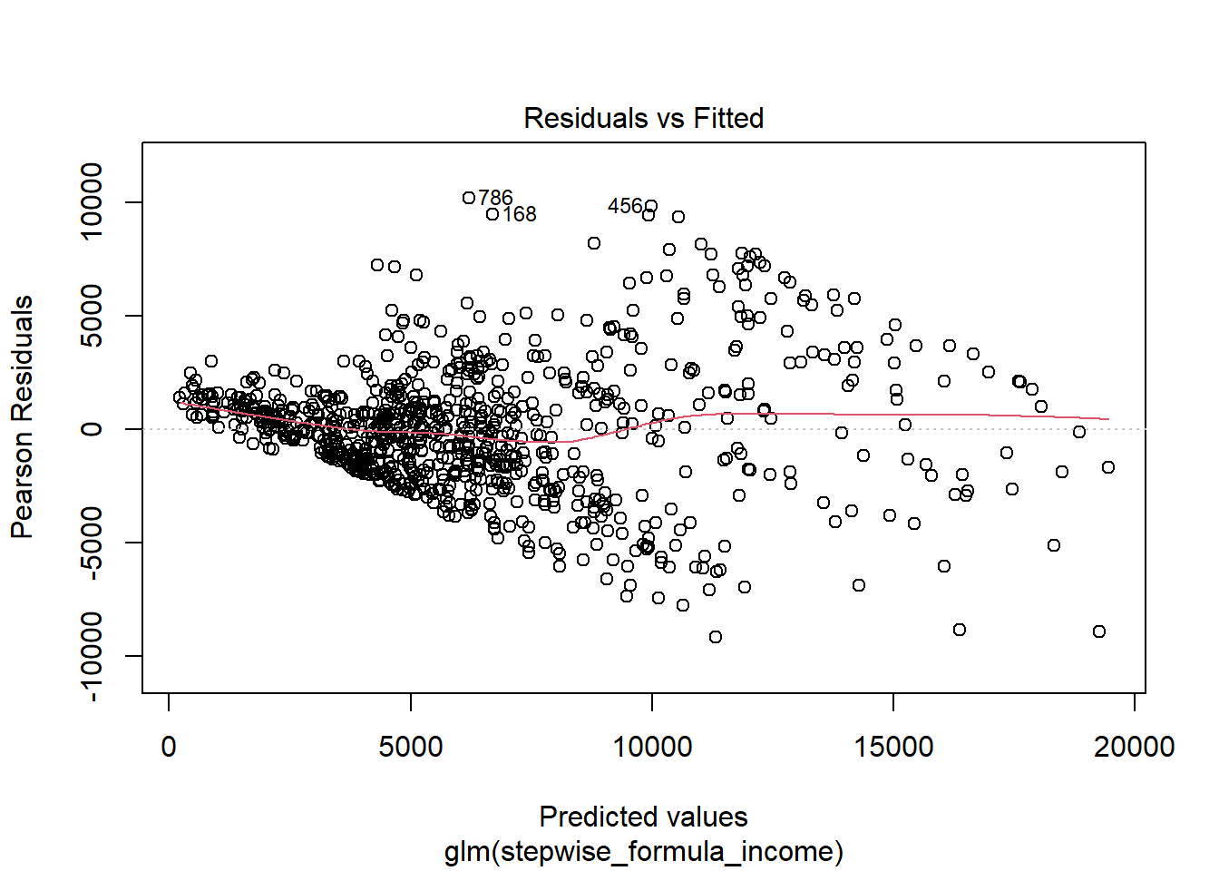
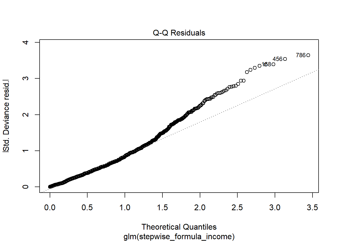
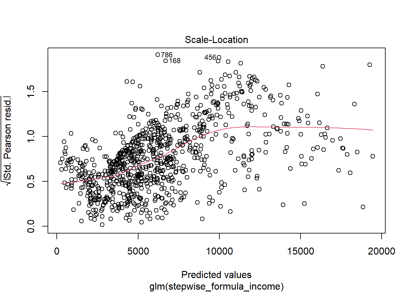
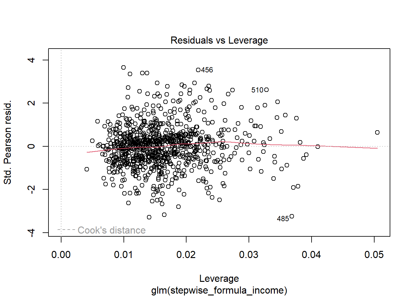
training_set_income <- attrition_Data3
testing_set_income <- attrition_Data_no_attrition


# The results of the stepwise analysis
stepwise_formula_income_reduced <- MonthlyIncome ~ TotalWorkingYears    +
   NumCompaniesWorked + YearsSinceLastPromotion

# reduced to significant
stepwise_formula_income <- MonthlyIncome ~ OverTime + JobInvolvement + TotalWorkingYears    +
    JobSatisfaction + StockOptionLevel+  NumCompaniesWorked + EnvironmentSatisfaction +
  YearsSinceLastPromotion + Department + JobRole + DistanceFromHome + EducationField +
  TrainingTimesLastYear + HourlyRate

# Build a linear regression model to predict MonthlyIncome
income_model <- lm(stepwise_formula_income, data = training_set_income)

summary(income_model)
##
## Call:
## lm(formula = stepwise_formula_income, data = training_set_income)
##
## Residuals:
## Min 1Q Median 3Q Max
## -9223.0 -1623.5 43.6 1341.4 10312.9
##
## Coefficients:
## Estimate Std. Error t value Pr(>|t|)
## (Intercept) 2706.709 814.330 3.324 0.000926 ***
## OverTime -107.466 212.336 -0.506 0.612909
## JobInvolvement 30.549 137.198 0.223 0.823848
## TotalWorkingYears 490.301 15.165 32.332 < 2e-16 ***
## JobSatisfaction -91.995 86.505 -1.063 0.287872
## StockOptionLevel -38.854 112.264 -0.346 0.729358
## NumCompaniesWorked -115.471 40.442 -2.855 0.004405 **
## EnvironmentSatisfaction 11.288 87.527 0.129 0.897413
## YearsSinceLastPromotion -77.761 34.419 -2.259 0.024120 *
## Department 264.643 222.766 1.188 0.235167
## JobRole -259.079 41.988 -6.170 1.05e-09 ***
## DistanceFromHome -8.928 11.853 -0.753 0.451549
## EducationField 63.764 74.217 0.859 0.390500
## TrainingTimesLastYear -7.696 75.853 -0.101 0.919208
## HourlyRate -4.064 4.793 -0.848 0.396711
## ---
## Signif. codes: 0 '***' 0.001 '**' 0.01 '*' 0.05 '.' 0.1 ' ' 1
##
## Residual standard error: 2812 on 855 degrees of freedom
## Multiple R-squared: 0.6321, Adjusted R-squared: 0.626
## F-statistic: 104.9 on 14 and 855 DF, p-value: < 2.2e-16# Predict MonthlyIncome for testing_set_income
predictions <- predict(income_model, newdata = testing_set_income)
# Add predicted MonthlyIncome to testing_set_income
testing_set_income$MonthlyIncome <- predictions
# Get the residuals from the model
residuals <- resid(income_model)
# Calculate RMSE
n <- length(residuals) # Number of observations
mse <- sum(residuals^2) / n # Mean Squared Error (MSE)
rmse <- sqrt(mse) # Root Mean Squared Error (RMSE)
print(paste("Root Mean Squared Error (RMSE):", rmse))## [1] "Root Mean Squared Error (RMSE): 2787.29937617916"# Copy Path
income_copy_Path <- "D:/University/SMU/Doing_Data_Science/DDS_repository/DDS_Final_project/CaseStudy2DDS/Attrition_Datasets/attrition_Data_no_income_with_predictions.csv"
# Save the updated dataset
write.csv(testing_set_income, file = income_copy_Path, row.names = FALSE)